Chapter 12 Time Course Analysis Module
This module finds genes whose expression changes over time, groups them by the shape of their time pattern, and finds genes that follow the same pattern as a gene of interest. Any sample attribute with ordered levels can be used as the time variable. The Mouse Microglia demo dataset has no real time series, but its three ages (2mo, 1yr and 2yr) can be used as time points, and Genotype can be used as the condition. The module has three tabs, described below: Time-Series DE Analysis (Section 12.1), DEG Clustering Analysis (12.2) and Similar Pattern Search (12.3). The analysis uses the samples selected in the “Groups and Samples” module (Chapter 3). Each tab has a green link that opens a short guide to its method.
12.1 Time-Series DE Analysis
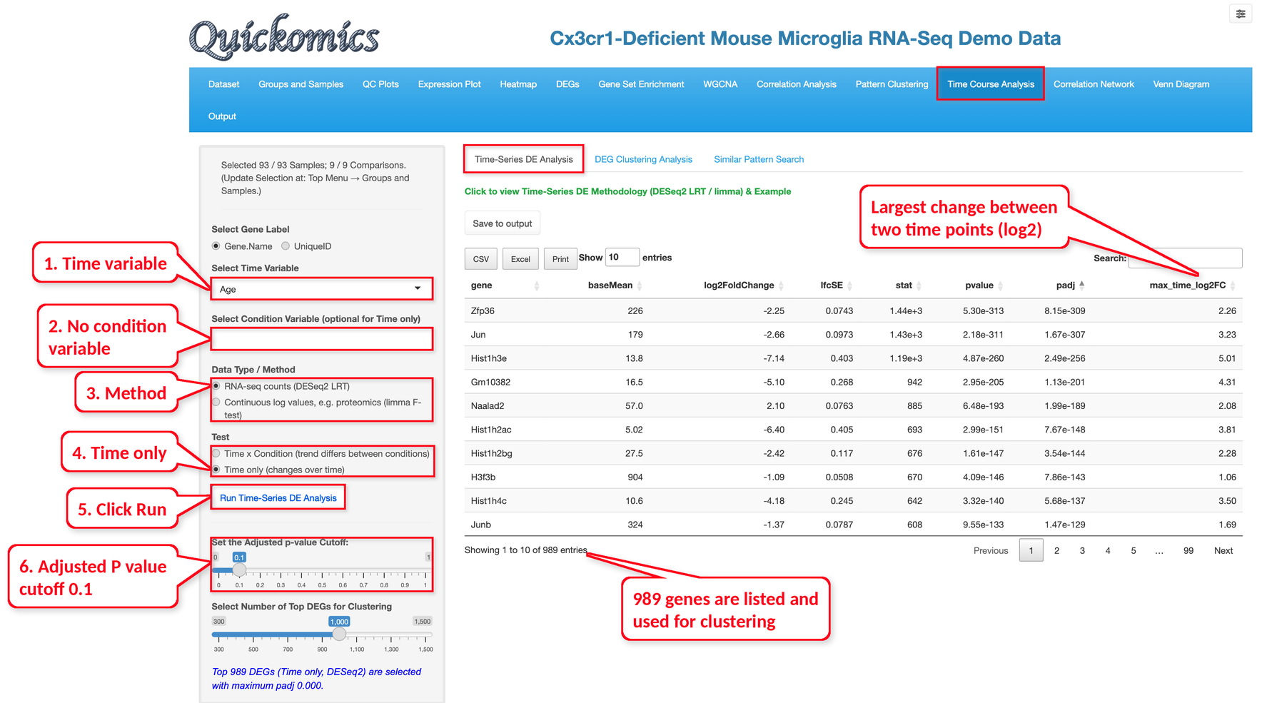
Select the time variable and, optionally, one or more condition variables, then choose the method and the test and click “Run Time-Series DE Analysis”.
Two methods are offered: a DESeq2 likelihood ratio test (LRT) for RNA-seq counts and a limma F-test for continuous log values such as proteomics data; the default is chosen from the expression unit of the project. Because the raw read counts are usually not available in Quickomics, the DESeq2 method converts the log expression values (for example log2(TPM+1)) back to the linear scale, using the log base and the small value taken from the expression unit of the project (2 and 1 when the unit does not give them), rounds them to whole numbers and treats these TPM-like values as counts. The results are therefore an approximation of a count-based analysis. For limma, “Min. Non-missing Values per Condition x Time Group” (2 by default) sets how many values each condition and time point needs. Two tests are offered. “Time x Condition” (the default) finds genes whose trend over time is different between the conditions, and “Time only” finds genes that change over time. Unlike the DEG module, the P values describe the whole trend of a gene, not a single fold change between two groups.
In the example below, we used Age as the time variable, no condition variable, the DESeq2 method and the Time only test, so the analysis asks which genes change with age in all samples together. Many genes change with age. The genes with the smallest adjusted P values below the cutoff of 0.1 are listed, up to the number set in “Select Number of Top DEGs for Clustering” (1,000 by default, 300 to 1,500); here 989 genes are listed, all with adjusted P values far below 0.1. The max_time_log2FC column gives the log2 fold change between the time points with the highest and the lowest mean expression. The top gene, Zfp36, has the smallest P value and a max_time_log2FC of 2.26. The table can be saved with “Save to output”.
12.2 DEG Clustering Analysis
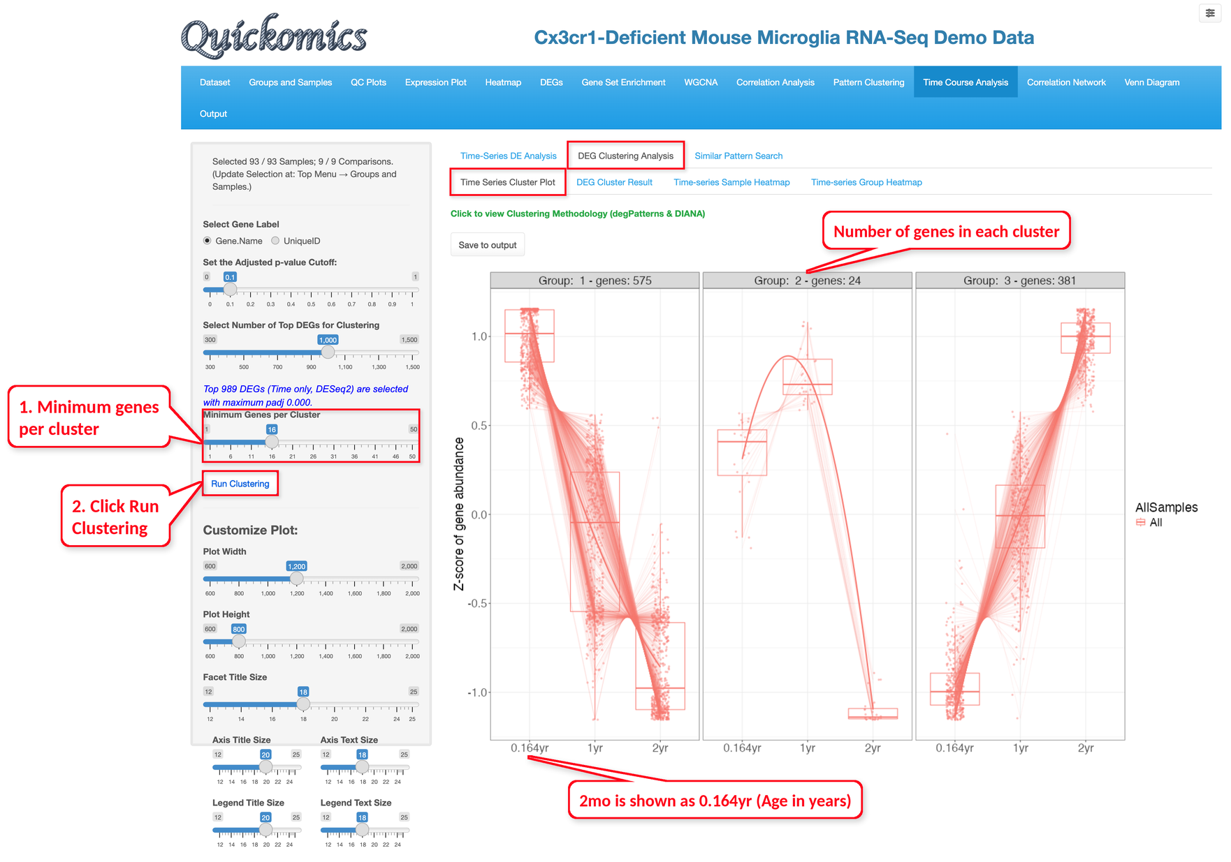
This tab groups the significant genes from Section 12.1 into clusters of genes with the same time pattern. The clusters are found with the degPatterns function of the DEGreport package, which chooses the number of clusters itself. Set the “Minimum Genes per Cluster” (16 by default) and click “Run Clustering”; smaller clusters are left out, so this number may need to be lowered when there are few significant genes.
The “Time Series Cluster Plot” sub-tab shows one panel per cluster, with the number of genes in its title. The box plots show the expression of the genes in the cluster at each age, scaled as z-scores, and the line shows the trend; when a condition variable is used, there is one box and one line per condition. Note that the plot gives the ages in years, so 2mo is shown as 0.164yr.
In the example below, 980 of the 989 genes fall into three clusters. The 575 genes of cluster 1 are highest at 2mo and decrease with age. The 381 genes of cluster 3 show the opposite pattern and are highest at 2yr. The 24 genes of cluster 2 go up from 2mo to 1yr and drop at 2yr.
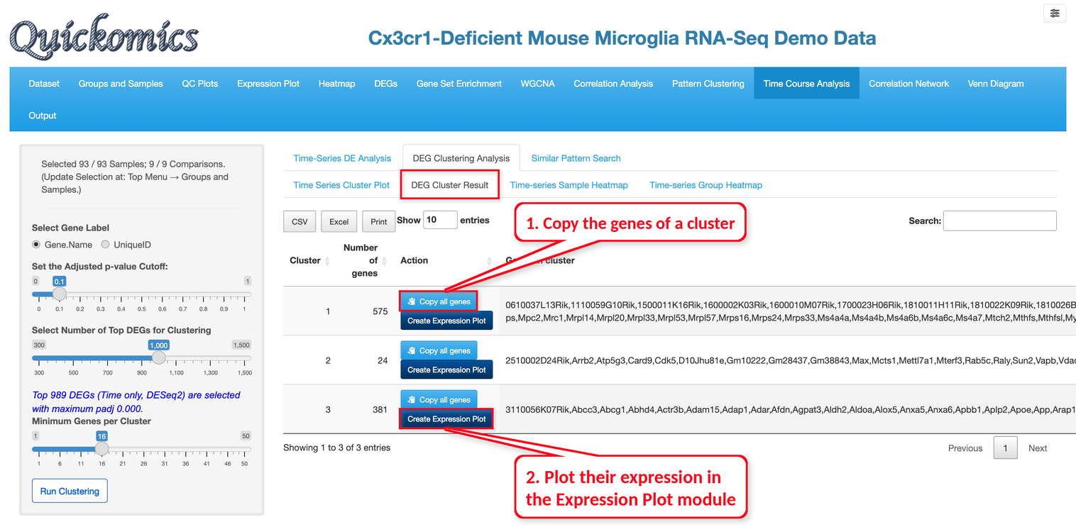
The “DEG Cluster Result” sub-tab lists the genes of each cluster. “Copy all genes” copies them so they can be pasted into other modules, and “Create Expression Plot” shows their expression in the Expression Plot module (Chapter 5).
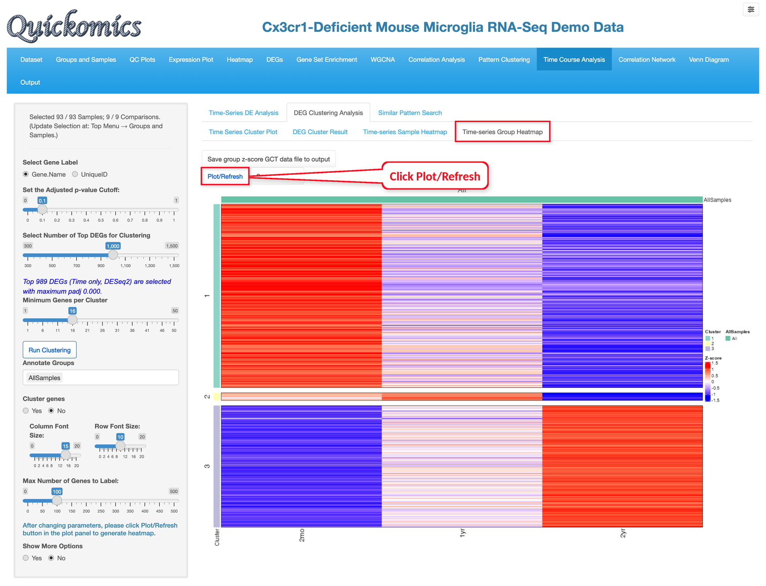
The “Time-series Sample Heatmap” and “Time-series Group Heatmap” sub-tabs show the genes of the clusters as heatmaps, one column per sample or one column per group. The samples or groups can be annotated with sample attributes (“Annotate Samples” or “Annotate Groups”), the genes can be clustered within each cluster (“Cluster genes”), and “Show More Options” sets the annotation colors, heatmap height and titles. Click “Plot/Refresh” to draw the heatmap after changing the settings. In the group heatmap below, the columns are the three ages, and the rows are the genes, split by cluster. Cluster 1 is red at 2mo and blue at 2yr, and cluster 3 is the reverse. The data behind each heatmap can be saved as a GCT file with the buttons above it.
12.3 Similar Pattern Search
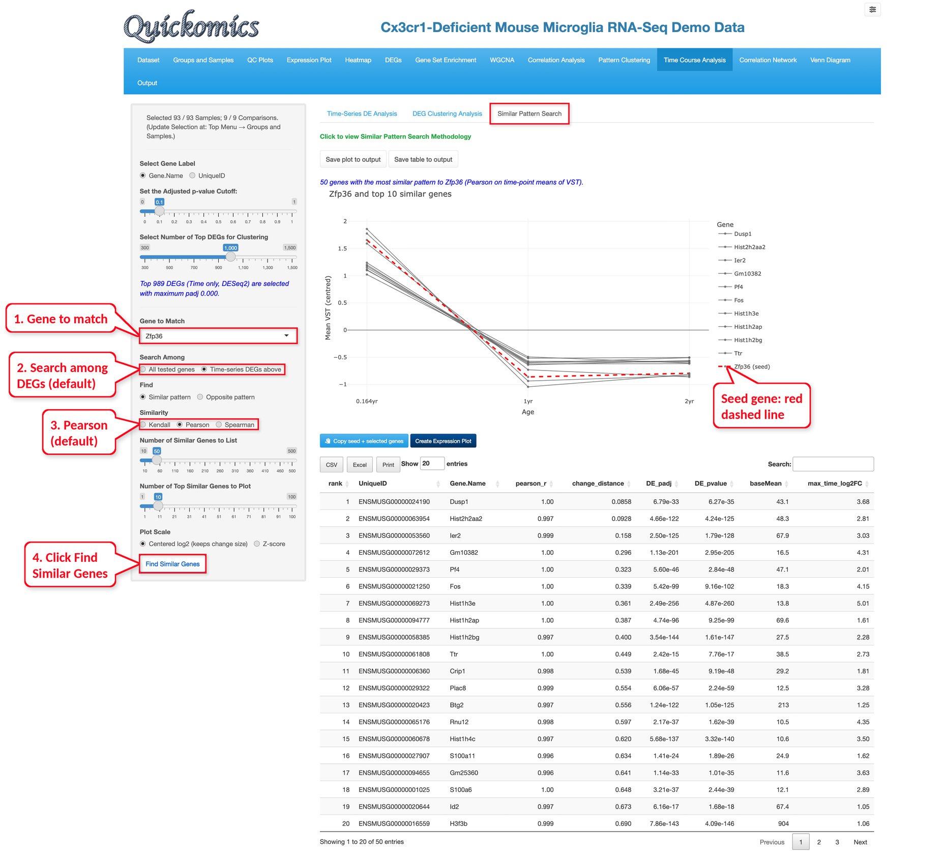
This tab finds genes whose expression changes over time in the same way as a chosen gene, or in the opposite way.
Run the Time-Series DE Analysis first, then type a gene in “Gene to Match”, choose whether to search only among the significant genes (the default) or among all tested genes, choose “Similar pattern” or “Opposite pattern” and the similarity measure (Kendall, Pearson or Spearman; Pearson by default), and click “Find Similar Genes”. By default, the 50 most similar genes are listed (“Number of Similar Genes to List”) and the top 10 are plotted (“Number of Top Similar Genes to Plot”). “Plot Scale” shows the values as centred log2 values, which keep the size of the changes (the default), or as z-scores. The plot shows the mean expression of the chosen gene, the seed gene, as a red dashed line, together with the most similar genes, for each condition and time point.
The table ranks the genes by how well their pattern matches the seed gene (pearson_r with the default Pearson similarity, where 1 is a perfect match); change_distance shows how close the size of the changes is, with smaller values meaning closer to the seed gene, and DE_padj and DE_pvalue give the adjusted and the raw P value of the gene from Section 12.1. A blank DE_padj means that DESeq2 left the gene out of the adjustment because of its low counts; DE_pvalue can then be checked instead.
In the example below, we searched the significant genes for genes similar to Zfp36. The top genes, such as Dusp1, Hist2h2aa2, Ier2 and Fos, are also high at 2mo and lower at 1yr and 2yr, with pearson_r close to 1. “Copy seed + selected genes” and “Create Expression Plot” pass the genes to other modules, and the plot and table can be saved to the output.