Chapter 2 Dataset Module
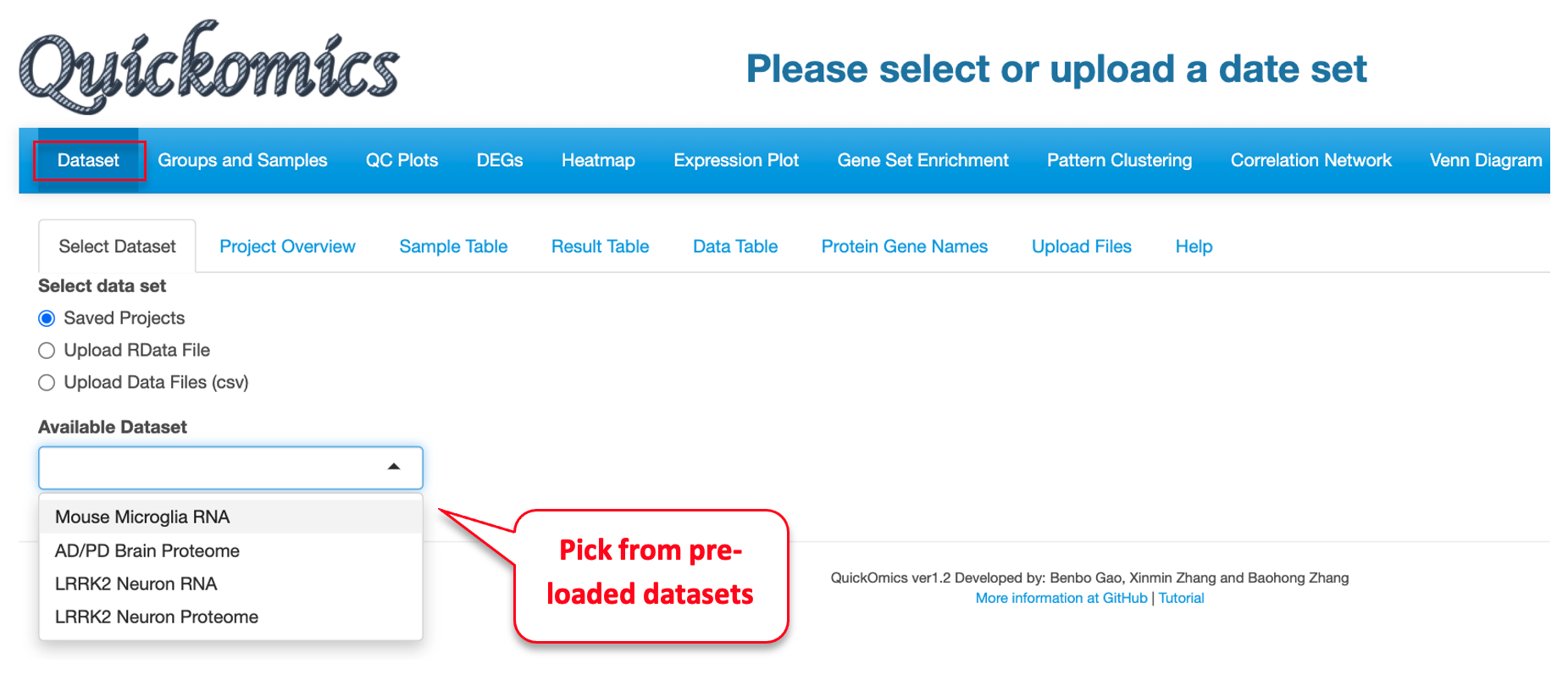
This first module is for selecting dataset. Users can either select from pre-loaded example datasets or upload their own dataset in a pre-defined format as detailed in section 2.1 and in our GitHub page (https://github.com/interactivereport/Quickomics). We have pre-loaded four datasets from published studies that users can use for demonstrative purposes. These includes two RNAseq datasets from Gyoneva et al., 2019 and Connor-Robson et al., 2019; and two proteomics datasets from Connor-Robson et al., 2019. Users can walk through multiple sub-tabs to visualize, select and download figures or data.
2.1 Upload Files
For a data set, the “Upload Files” tool allows users to upload three required files, namely sample metadata, normalized expression data and statistical comparison results in csv format (Comma Separated Values) to Quickomics directly. Example data sets are provided in GitHub for both RNAseq (https://bit.ly/2MRkFcb) and proteomics (https://bit.ly/3rn4i6a). Detailed formatting guidance is outlined below,
- Sample Metadata File: It should have “sampleid” and “group” columns, with additional columns optional. Sample identifiers must match those used in the expression data file.
- Expression Data File: It should be a matrix of expression values with genes/proteins as rows, and samples as columns. The unique IDs for genes/proteins are in the first column. We recommend using log of normalized expression values, e.g. log2(TPM+1) for RNAseq data or normalized intensity or ratio for proteomics data.
- Comparison Data File: It should have five columns, “UniqueID”, “test”, “Adj.P.Value”, “P.Value” and “logFC”. The comparison names are listed in “test” column. Please note that wrongly named column headers will cause issues.
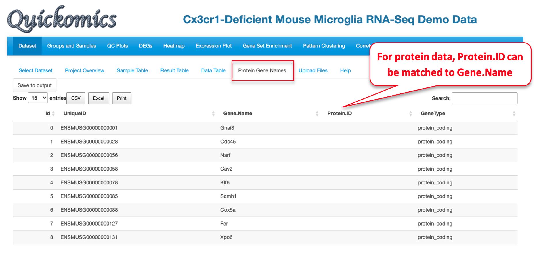
- Optional Gene/Protein Name File: The system has built-in function to convert unique IDs in the data files to gene symbols and create the Gene/Protein Name file, so most users don’t need to prepare the file. Nevertheless, if provided by users, it must have four columns: “id” (sequential numbers like 1,2,3 … …), “UniqueID” (matching IDs used in the expression and comparison data file), “Gene.Name” (official gene symbols), “Protein.ID” (UniProt protein IDs, or keep it empty for RNA-Seq data). Additional columns (e.g. gene biotype) are optional.
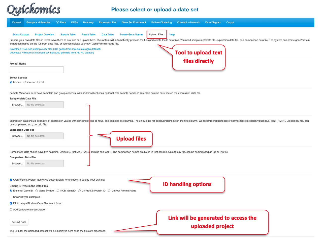
After the data files are processed, Quickomics will automatically load all required data for exploration immediately and provide a link for the user to come back in the future.
Behind the scene, Bioconductor biomaRt package (https://bioconductor.org/packages/release/bioc/html/biomaRt.html) has been used to convert gene IDs (Ensembl gene, NCBI gene ID, etc.) into gene symbols by querying Ensembl databases. For protein IDs, we generated a custom lookup table using information downloaded from UniProt Knowledgebase to convert UniProt IDs to gene symbols and protein names. We didn’t use biomaRt for proteins as Ensembl databases only cover about 60-80% protein IDs in a typical proteomics data set.
2.2 Prepare R Data Files by Computational Biologists
We recommend uploading csv files, which is convenient for general users who can skip section 2.2 entirely. Nevertheless, experienced R programmers can create R data files to be uploaded through “Upload RData File” option. Section 2.2.1 and 2.2.2 provide example R scripts to prepare such R data files for RNA-Seq and proteomics data, respectively.
Two R data files are required for each data set, one contains the main data and the other contains gene co-expression network information. For the pre-loaded datasets, main data files are located in the “data” folder, https://github.com/interactivereport/Quickomics/tree/master/data, and gene co-expression network files are located in the “networkdata” folder, https://github.com/interactivereport/Quickomics/tree/master/networkdata. One can review the content of a R data file (e.g. Mouse_microglia_RNA-Seq.RData) in the “data” folder by loading it into R. The main R data file contains the following R data frame objects.
- MetaData: It must have “sampleid”, “group”, “Order” and “ComparePairs” columns. Additional metadata columns about samples are optional. “sampleid” should match those used in expression data. “group” holds group names of samples. “Order” is ordered group names used on plotting. “ComparePairs” are names of comparisons performed.
- ProteinGeneName: It must have “UniqueID”, “Gene.Name” and “Protein.ID” columns. “UniqueID” matches gene ID in below data_wide and data_long objects. “Gene.Name” should be official gene symbols. “Protein.ID” is UniProt protein IDs, or empty for RNA-Seq data. Additional columns about proteins or genes are optional.
- data_wide: This is the expression matrix in which rows are genes and columns are samples. Samples must match “sampleid” values in MetaData and gene IDs must match “UniqueID” values in ProteinGeneName.
- data_long: Gene expression matrix in long format with four columns, “UniqueID”, “sampleid”, “expr” and “group”. “group” values must match those listed in MetaData.
- results_long: The comparison results in long format with five columns, “UniqueID”, “test”, “Adj.P.Value”, “P.Value” and “logFC”. “UniqueID” matches “UniqueID” in ProteinGeneName. “test” column has the comparison names that must match “ComparePairs” values in MetaData. The other values are typically computed from statistical analysis, but the data headers must be changed to “Adj.P.Value”, “P.Value” and “logFC”.
- data_results: This is a summary table starting with “UniqueID” and “Gene.Name” columns, then the intensity (max or mean expression value from data_wide for each gene), mean and SD expression values for each group, and finally comparison data (comparison name added as prefix of columns).
The network data object is computed from “data_wide” expression matrix by using Hmisc R package exemplified by the code snippet below.
cor_res <- Hmisc::rcorr(as.matrix(t(data_wide)))
cormat <- cor_res$r
pmat <- cor_res$P
ut <- upper.tri(cormat)
network <- tibble::tibble (
  from = rownames(cormat)[row(cormat)[ut]],
  to = rownames(cormat)[col(cormat)[ut]],
  cor = signif(cormat[ut], 2),
  p = signif(pmat[ut], 2),
  direction = as.integer(sign(cormat[ut]))
)
2.2.1 Example R script to prepare R data files from RNA-Seq results
We have provided example input files (TPM and count matrix files, sample grouping file, comparison list file) and the R scripts to generate the main data and network R data files at https://github.com/interactivereport/Quickomics/tree/master/demo_files/Example_RNA_Seq_data. Please note that you may need to modify RNA_Seq_raw2quickomics.R to fit your input files. • rsem_TPM.txt: The TPM matrix. One can also use RPKM matrix if needed. • rsem_expected_count.txt: The gene count matrix. We used RSEM counts in this case, but gene count results from other methods can be used as well. • grpID.txt: This file lists the group information for each sample. • comparison.txt: This list lists the comparisons to perform (group 1 vs group 2 in each row). The following command will read the above data files, run differential gene expression analysis using DESeq2, and create main and network R data files.
$ Rscript RNA_Seq_raw2quickomics.R2.2.2 Example R script to prepare R data files from proteomics results
We have provided the example input files (normalized protein expression, comparison data, sample information, protein and gene names) and the R script to generate the main data and network R data files at https://github.com/interactivereport/Quickomics/tree/master/demo_files/Example_Proteomics_data. Please note that you may need to modify Proteomics2Quickomics.R to fit your input files.
• NormalizedExpression.csv: Normalized protein expression (log2 transformed).
• ComparisonData.csv: Comparison results. The statistic values are: logFC, P.Value and Adj.P.Value. This can be created using R packages like limma.
• Sample.csv: Sample information file.
• ProteinID_Symbol.csv: This file lists the proteinIDs and associate gene symbols. The following command will read the above data files and create main and network R data files.
$ Rscript Proteomics2Quickomics.R2.3 Sample Table
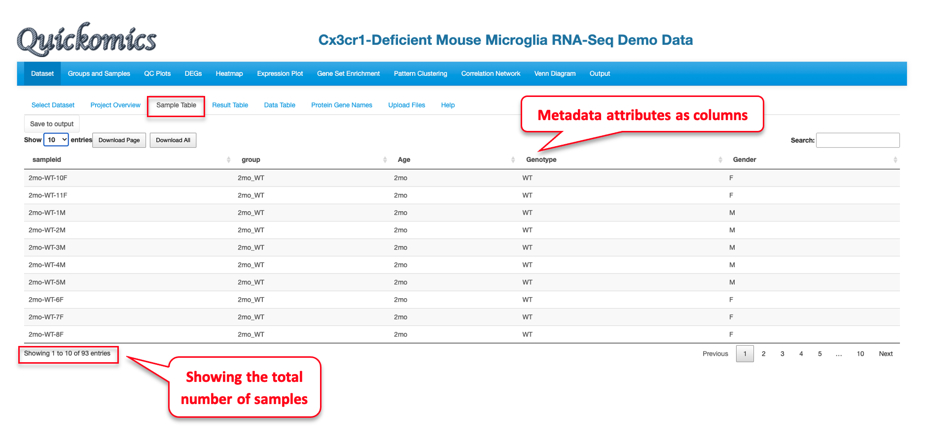
A sample table with metadata/details appears upon completion of dataset loading. Here we have selected the “Mouse Microglia RNA” dataset from the previously published paper (Gyoneva et al., 2019) as an example to illustrate all the functionalities. This publication used RNAseq to conclude that the knockout of the Cx3cr1 gene altered the microglial transcriptome in a manner similar to what ageing does, albeit in a milder extent. Using Quickomics, we can visualize the original results from the paper, as well as provide novel visualizations to support new results.
The Sample Table contains detailed info of all study samples. A total of 93 samples that were sequenced in this project are listed in the table with attributes like sampleid, group, Age, Genotype and Gender, shown in different columns.
2.4 Project Overview
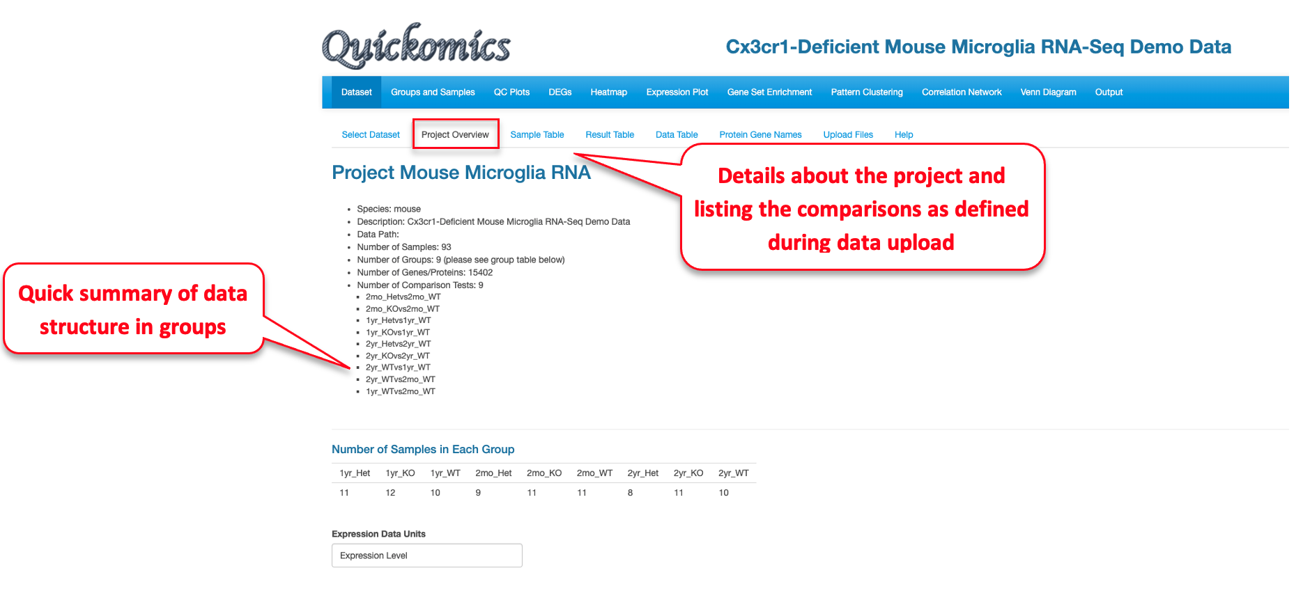
This tab gives an overview of all samples in the project by providing a summary from the metadata. This includes information like which species was used, the different comparisons run and total number of samples in each group. This tab also helps identify how many groups were present in the dataset, like in this project there are 9 different groups that correspond to three genotypes in each of three time points (WT, Het, KO; 2mo, 1yr, 2yr).
2.5 Result Table
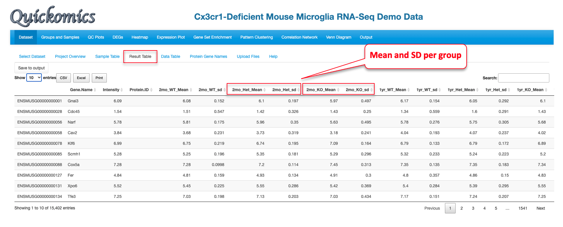
This tab contains statistical analysis results like Ensemble ID (for RNAseq data) and Accession ID (for proteomics data), gene name, mRNA or protein abundance (count or intensity), mean and SD values for each group, log2 fold change, P value and adjusted P value.
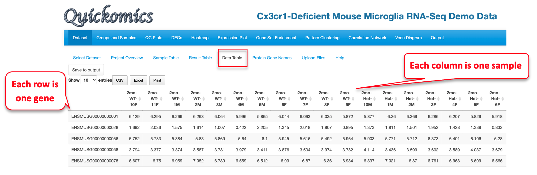
2.6 Data Table
The Data table contains normalized expression values (TPM for RNAseq, intensity for label free proteomic quantification, or ratio for isobaric label proteomics quantification) per sample for each gene. In Quickomics version 2.0, we added “Download all” button for small tables, and enable “Save to output” button for large tables.