Chapter 7 Running the pipeline
If you would like to perform ambient RNA removal using CellBender, please follow the instruction here to run scRMambient first. The scRMambient pipeline will run CellBender based on unfiltered h5 input files and created new h5 files to run scAnalyzer. We have a detailed tutorial.
After preparing the input data and configuration files (config.yml and sampleMeta.csv), we are ready to run the pipeline. Please be aware that scRNASequest is a semi-automated pipeline, and certain steps require the user to review the outputs and determine the parameters. Thus, the same step may need to be run for more than once, especially for finaling the QC parameters.
7.1 Initial scAnalyzer run
The initial scAnalyzer run intends to test the default filtering parameters on the single-cell RNA-seq data. We suggest the following settings in the config.yml file to activate the filtering step, but pause the pipeline from additional analysis (such as data integration, harmonization, etc.):
# Change the following settings in the config.yml file:
filter_step: True
runAnalysis: False
To run scAnalyzer, simply pass the path to the config.yml file to the program:
scAnalyzer Path/to/a/config/file

#Example:
scAnalyzer ~/E-MTAB-11115/processing/config.yml
Output files:
outputdir
    ├── BookdownReport/                #Full bookdown report folder. This is same as the BookdownReport.tar.gz below
    ├── config.yml
    ├── config.yml.20220617.log        #log file
    ├── ProjName_BookdownReport.tar.gz #Bookdown report tar ball.
                                       #Please download this file and open the index.html file to view the report
    ├── ProjName_raw_prefilter.h5ad    #h5ad after pre-filtering
    ├── prefilter.QC.pdf               #QC plots before filtering. These plots are included in the Bookdown report
    ├── postfilter.QC.pdf              #QC plots after filtering
    └── Rmarkdown/                     #Source files for the Bookdown report
7.2 Review the bookdown report
After the initial scAnalyzer run, a bookdown report, named ProjName_BookdownReport.tar.gz will be generated. Please open the report (index.html) to review cell numbers and figures before and after the filtering step, and adjust the following thresholds in the config.yml file if needed:
# Cell filtering parameters in the config.yml file:
gene_group:
  MT:
    startwith: ["MT-","Mt-","mt-"]
    cutoff: 20           #percentage cutoff to filter out the cells (larger than this cutoff)
    rm: False
  RP:                    #for ribosomal genes if you would like to filter them
    startwith: []
    cutoff: 20
    rm: False
filter_step: True        #if False, the above 'gene_group' filtering will be skipped as well
min.cells: 3             #filtering genes by minimum number of cells with non-zero count for a gene
min.features: 50         #filtering cells by minimal genes detected
highCount.cutoff: 10000  #any cells with higher total counts to be removed
highGene.cutoff: 3000    #any cells with a higher number of detected genes to be removed
The min.cells cutoff is to filter out genes that have low representation in cells, and the min.features cutoff is to filter out cells that have low number of genes (features) detected. The last two cutoffs, highCount.cutoff and highGene.cutoff can be used to filter cells if they have too many total counts or UMI detected, possibly due to multiplets. Please evaluate these cutoffs carefully, because the default values here may not be suitable for all datasets.
The user may need to adjust the thresholds and rerun scAnalyzer to visualize the results. This step may be repeated until the threshold is adequate for the data.
Please find an example of the bookdown report here: E-MTAB-11115 bookdown
7.3 Generate a slide deck
This is an optional step if you have already reviewed the Bookdown report. This slide deck is another way to organize and present the same results.
The QC report can be turned into a online slide deck format for better sharing and demonstration. To achieve this, please use the Slidedeck.Rmd file under the /src folder and follow the steps below:
# create a new directory inside the project, and link the existed files and folder:
cd ~/E-MTAB-11115/processing/
mkdir Slidedeck && cd Slidedeck
ln -s ../BookdownReport/images
ln -s ../BookdownReport/bookdown.info.txt

# Copy the Slidedeck.Rmd file from src directory to the working directory containing config.yml file.
# We assume your pipeline was installed under ~/scRNAsequest/
cp ~/scRNAsequest/src/Slidedeck.Rmd ~/E-MTAB-11115/processing/Slidedeck

# Source the environment
src="~/scRNAsequest/src"
source $src/.env;eval $condaEnv

# Run the Slidedeck script, and set the output file name using 'output_file' parameter
Rscript -e 'rmarkdown::render("Slidedeck.Rmd", output_file="Output.html")'
Please download the whole Slidedeck directory and open the Output.html file in a web browser.
Please find an example of the bookdown report here: E-MTAB-11115 slidedeck
7.4 Doublet detection
Based on the recent benchmarking paper and single-cell RNA-seq analysis guideline, we implement scDblFinder in our pipeline to perform doublet detection. By default, the pipeline runs scDblFinder on each sample and produces doublet scores (0-1, higher means high probability to be doublet) and classification results (singlet or doublet) using its own cutoff. If you speculate ambient RNA contamination in your data, we also suggest running scRMambient first.
Users can control whether to remove these cells by setting dbl_filter in the config.yml file. False means not removing doublets, but the score (column name: scDblFinder.score) and classification (column name: scDblFinder.class) will be added to the final results for evaluation. If True, then all doublets will be removed.
dbl_filter: FalseThe scDblFinder automatically determines the doublet rates based on cell number, i.e., for N thousand cells, the doublet rate will be close to N %.
However, you can adjust this manually by providing a numeric number between 0~1 in the config.yml file to enforce your own cutoff on the doublet score:
dbl_filter: 0.957.5 Cell type label transfer
Cell type label transfer is to label our new data using a reference single-cell RNA-seq data from the same tissue (i.e. brain, muscle, etc.). It automatically assigns cell types to each single cell. scRNASequest pipeline can do this if you provide a reference in the config.yml file.
However, this is optional, so leaving ‘ref_name’ parameter as blank won’t affect running the pipeline. But we strongly suggest you perform label transfer to better understand the biology of the data.
To check all available references, run scAnalyzer without any parameter and they will be printed out on the screen if you have added any references using scRef, see section Reference building. Alternatively, you can provide your own reference in Azimuth format to the pipeline.
Example 1, if you have a named reference that has been added to the pipeline, for example, human_cortex is included already:
ref_name: human_cortexExample 2, if you have an rds with cell type labels, you can also provide a path to the reference file and use it to label the current dataset. In the demo dataset, we have a reference rds file prepared and you can use it directly:
ref_name: ~/scRNAsequest/rat_cortex_ref.rdsThe above rds file must be in Azimuth format, which can be prepared by running scRef.
7.6 Adjust major_cluster_rate
If you have turned on cell type label transfer by providing a reference dataset, you may consider adjusting major_cluster_rate in the config.yml file. This major cluster rate means the proportion (by default 0.7) of cells of an integration cluster to be assigned to a Seurat reference label.
In the final cell type labels, the predicted.celltype is the the labels predicted by Seurat label transfer. The following predicted labels: liger_cluster_predicted.celltype, normalized.louvain_predicted.celltype, raw.louvain_predicted.celltype, and sctHarmony_cluster.predicted.celltype are re-labelled cell types considering dimension reduction/integration clusters. The dimension reduction/integration algorithms generate numeric clusters, and our pipeline will look through each cluster and check if over 0.7 (by default, 70%) of the cells belong to one label. If yes, the whole cluster will be assigned to that cell type label. If not, it will leave that numeric cluster in the final result. We can consider those numeric labeling as a mixture or ‘Unclassified’ cell types.
So, if you find cell type labels with just numbers and you don’t want to see them (The numbers indicating original cluster id whose cells belong to any label is lower than the threshold), you can turn this off by removing the default number 0.7 and leaving it empty like this in the config.yml file:
major_cluster_rate:7.7 Run the pipeline in parallel
As mentioned in the previous section Input configuration, users can choose sge or slurm based on your scheduler option in the config.yml file to run your jobs parallelly. For large datasets, we highly recommend that users make full use of the CPU parallelization. Here is an example of using 8 cores on slurm HPC scheduler, in the config.yml file:
parallel: slurm              #False by default. Use 'slurm' for Edge cluster, and use 'sge' for Cambridge HPC
core: 8                      #Number of cores to use
If you don’t have sge or slurm scheduler, simply use ‘parallel: False’ as default.
7.8 Run the full analysis
We have finalized the filtering criteria and made necessary adjustment in the config.yml file to set up label transfer, major_cluster_rate, and parallelization.
Now, we are ready to turn on the runAnalysis parameter in the config.yml and run the full pipeline:
# Change the following setting in the config.yml file:
runAnalysis: True
overwrite: True    #Overwrite the previous results if we run this again, for example, after adjusting some parameters.
You can always go to our demo dataset to review related data and demo config.yml settings.
Then run the following command again:
scAnalyzer Path/to/a/config/file

#Example:
scAnalyzer ~/E-MTAB-11115/processing/config.yml
This step will be time-consuming, and it took ~1 hour for the E-MTAB-11115 data (final cell number: 29,511) to finish. For a larger dataset with 110k cells we have tested, the full pipeline took ~7 hours.
7.9 Visualize the harmonized results
After running the pipeline, you will see the following files in the working directory. Each harmonization method (Harmony, Seurat, Liger) will also generate corresponding files.
outputdir
# Input files
├── config.yml: The analysis config file specify the scAnalyzer parameters
├── sampleMeta.csv: List all sample information including expression matrix (and sample/cell level meta information)
└── DEGinfo.csv: Define the sc DEG (between phenotypes within a cluster annotatino)
# Main results under the output dir:
├── [prj_name].h5ad: The final h5ad file which is used for cellxgene VIP loading (will be copied into the celldepotDir folder set by sys.yml)
├── [prj_name].db: The final db file which is used for cellxgene VIP loading (will be copied into the celldepotDir folder set by sys.yml)
├── [prj_name].h5seurat: The h5seurat file of the final results
└── [prj_name]_raw_added.h5ad: The h5ad file contains raw counts in X along with all annotation and embeding
(will be copied into celldepot folder)
# Rmarkdown:
├── Rmarkdown: The folder contains png files for R bookdown
├── [prj_name]_BookdownReport.tar.gz: R bookdown document tarball for downloading and sharing
└── BookdownReport: The folder contains R bookdown reports
# Log file:
└── config.yml.[date].log: All stdout/stderr will be recorded in this dated log file
└── [Software].error: Standard error files of multiple software, including:
Harmony, Liger, SeuratRPCA, SeuratRef, SCT, sctHarmony, silhouette, etc.
These files will be under the log/ directory if you did not run in the parallel mode
These files will be under the j[numeric] folder if you ran the pipeline in the parallel mode
# QC files under the QC/ folder:
├── sequencingQC.csv: Merged all sequence QC files from individual samples if available
├── sequencingQC.pdf: Plots of sequence QC if they are available
├── prefilter.QC.pdf: Initial data QC plots without filtering
└── postfilter.QC.pdf: Data QC plots after filtering
# evaluation folder for harmonization evaluation:
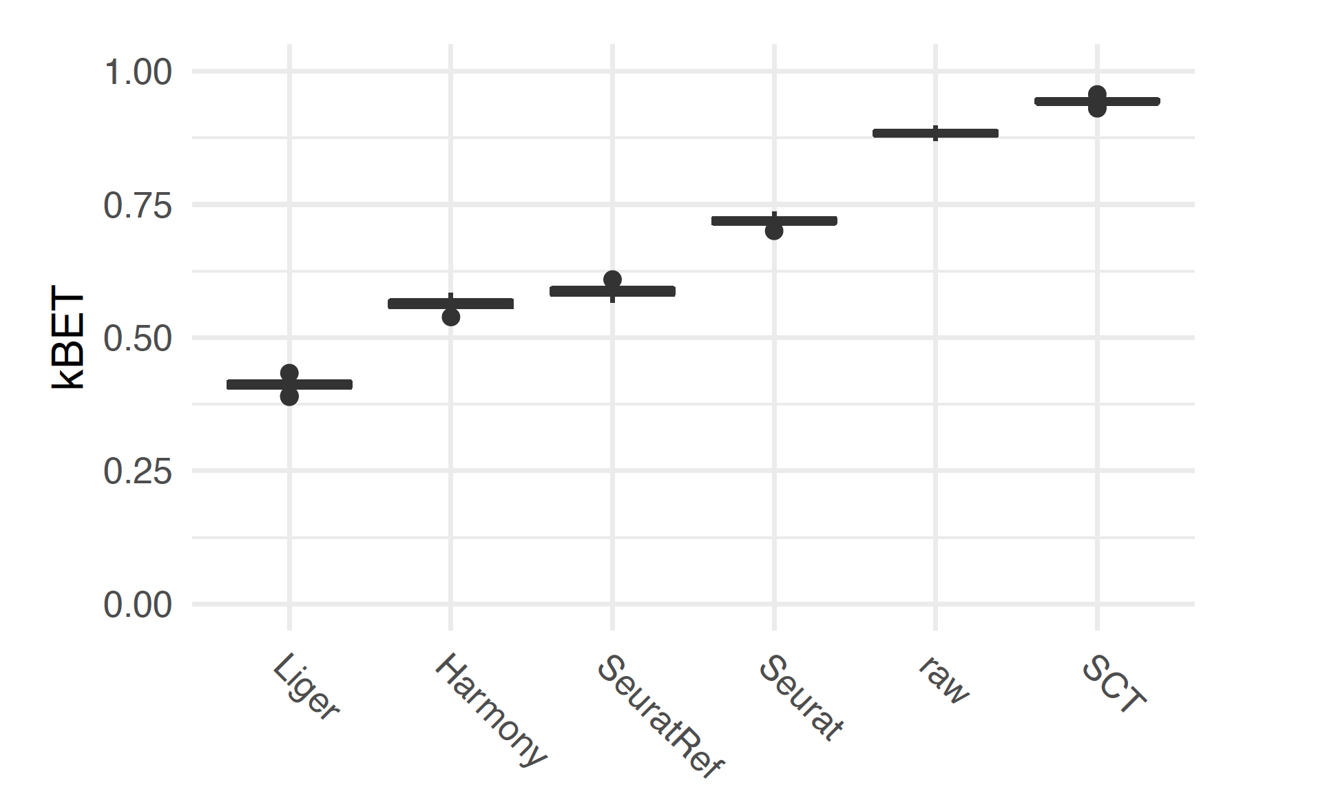
├── [prj_name]_kBET_umap_k0_100.pdf The kBET evaluation plot for all integration methods
└── [prj_name]_Silhouette_boxplot_pc50.pdf The Silhouette evaluation plot for all integration methods
# raw/ folder for h5ad files before and after QC, but have not run through the pipeline:
├── [prj_name]_raw_prefilter.h5ad: The internal temporary raw counts created/merged directly from sample before filtering
└── [prj_name]_raw.h5ad: The internal temporary raw counts after the cell/gene filtering
# SCT/ folder:
├── [prj_name].h5: The sparse matrix contains SCT expression values
├── [prj_name].h5.rds: The Seurat object contains counts (RNA assay) and
SCT expression (SCT assay) along with original meta information from SampleMeta file
├── [prj_name].cID Cell barcodes
├── [prj_name].gID Gene ID
├── [prj_name].scalF Scale factor
└── [prj_name].h5ad: The SCT expression, along with PCA, tSNE, UMAP reduction layout, will be
merged into [prj_name].h5ad
# SeuratRPCA folder for Seurat RPCA integration results:
├── [prj_name].csv.gz: The reuction embedding and clustering results from seurat RPCA integration
└── [prj_name].h5ad: The seurat RPCA integration with reduction embedding and clustering,
will be merged into [prj_name].h5ad
# SeuratRef folder for Seurat reference mapping results:
├── [prj_name].csv: The reuction embedding and label transfer results from seurat RPCA integration
└── [prj_name].h5ad: The seurat reference mapping results with reduction embedding, will be merged into [prj_name].h5ad
# sctHarmony folder for Harmony based on SCT transformation:
├── [prj_name].csv: The PCA iinformation of each cell
└── [prj_name].h5ad: The harmony integration with reduction embedding and clustering,
will be merged into [prj_name].h5ad
# Liger folder for Liger integration results:
├── [prj_name]_hvg.csv: High variable gene list
├── [prj_name].csv: The liger integration embedding and cluster
└── [prj_name].h5ad": The liger integration with reduction embedding and clustering,
will be merged into [prj_name].h5ad
# [prj_name]_scDEG folder (if you ran the DEG step):
├── Comparisone names folders
├── .csv files for each cell type: The DEG analysis results
├── .rds files for each cell type: The rds data
└── .pnd files for each cell type: The volcano plots
# Parallel directory (if you ran the pipeline in parallel mode):
└── j[numeric]: A colder contains parallel jobs submit script and log filekBET is a useful metric to evaluate and compare the harmonization results. Here is an example of the ProjName_kBET_umap_k0_100.pdf result:
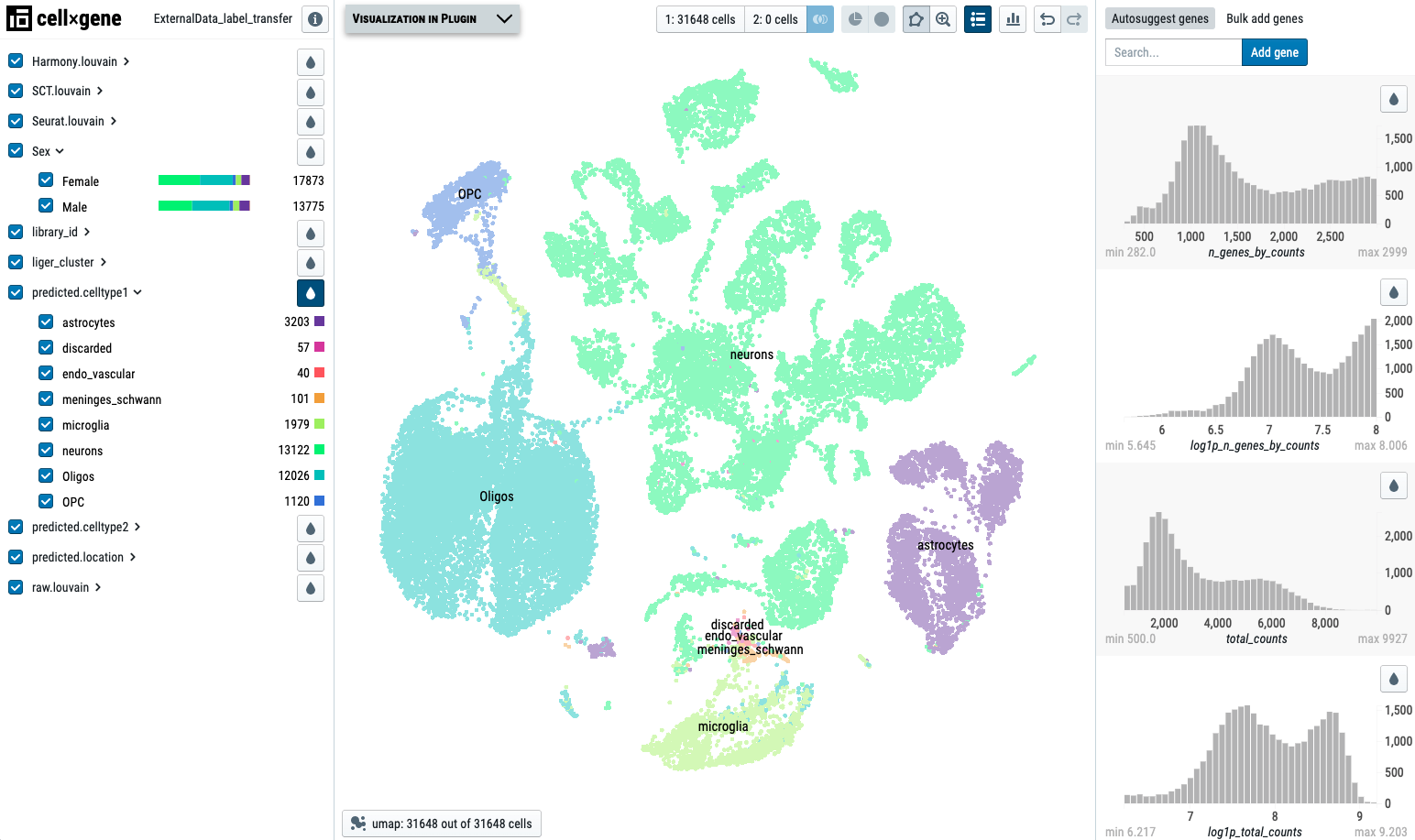
Please review the ProjName.h5ad file for the harmonization result. If you have Cellxgene VIP installed, the visualization will be easier.
Here is an example of the ProjName.h5ad project visualized by Cellxgene VIP:
Update on August 2023: covariate checking
Now the pipeline will also output two additional files for pair-wised correlation analysis of covariates in obs:
obsCor.csv: pair-wised p values
obsCor.pdf: all pair-wised plots
If both are numeric, a scatter plot with correlation test.
If one is numeric while the other is categorical, a boxplot with one-way anova test.
If both are categorical, a barplot (cell number) with chi-square test, and a contingency table will be plotted for these two categorical variables.