Chapter 8 Differential expression (DE) analysis
Another critical function of the scRNASequest pipeline is the Differential expression (DE) analysis. By running the steps in Section: Running the pipeline, we have performed quality control of the data, and generated an integrated dataset.
Before running the DE analysis, the DEGinfo.csv comparison file needs to be prepared:
![]()
The first column, comparisonName is designed to store the name of the comparison. These names will be used to create separate folders under the result directory. In the DEG comparison file above, “sample”, “cluster”, “group” and “covars” are the annotation headers, and “alt” and “ref” are the two entries from “group” column. The “covars” is optional and can be empty.
The DEG is performing between “alt” and “ref” cells from “group” within each entry of “cluster” considering “sample” variations. The “group” variable should contain conditions to compare, such as Mutant v.s. Control. Thus, this pipeline is designed to loop through each cluster, and perform DEG analysis between “alt” v.s. “ref”.
Covariate adjustment:
Adjusting covariates is optional. By default, NEBULA considers the value of log of total UMI (library size) as the offset covariate in our pipeline, so you don’t need to adjust this again in “covars”.
If needed, you can put a formula in the “covars” column using the meta information from the sampleMeta.csv file, such as Sex, Age, etc. You can also include QC metrics such as mitochondria percentage (pct_MT), etc. Please find a full list of QC metrics below. You can also open the Cellxgene VIP and check the right side. All numeric covariates are listed there.
n_genes_by_counts, log1p_n_genes_by_counts, pct_counts_in_top_50_genes, pct_counts_in_top_100_genes, pct_counts_in_top_200_genes, pct_counts_in_top_500_genes, pct_MT, n_genes, predicted.CellType.scoreYou may consider pct_MT as a covariate to adjust, but be careful to adjust other covariates here unless you have a good reason to do so. An example of the formula to be filled out in the “covars” column: Age+Sex+pct_MT.
Continuous/Numeric variable as the comparison group:
If the user is interested in using a numeric variable (such as Age) as the comparison group in the comparison, please provide the column header of the numeric column in the cell/sample meta table in the “group” column of the above DEGinfo.csv table, and leave “alt” and “ref” columns of that row empty. Currently this function is only supported if DE analysis is run using the NEBULA method.
Missing values:
It’s important to know that if any cells don’t have such DE condition information. For example, some samples don’t have information such as ‘treated’ or ‘control’ labeled, and instead, the values were ‘NA’, ‘NaN’, etc. In such case, we can easily include such information in the main config.yml file by defining the NA values to be ignored. The pipeline will remove all these cells from the DE analysis.
#An example of the config.yml file:
NAstring: [NA, NaN, NAN] #provide a list of strings which should be considered NA and associated cells to be removed
DE software choices:
Based on the previous benchmarking analysis, NEBULA outperforms other software in single-cell RNA-seq DE analysis. Thus, our pipeline uses NEBULA by default to run DE. However, we also offer the following methods as well, and you can directly use them in the DEGinfo.csv file, see Example 3 later.
u_test: Mann–Whitney U test, also called Wilcoxon rank-sum test, is a nonparametric test. See Wiki. In our single-cell RNA-seq analysis, this is a pseudobulk method.
t_test: Student’s t-test, statistical test based on Student’s t-distribution. See Wiki. In our single-cell RNA-seq analysis, this is a pseudobulk method.
edgeR: Using the edgeR package to perform pseudobulk DE analysis. Refer to their paper for more details.
limma: Using the limma-voom method to perform pseudobulk DE analysis. Refer to their paper for more details.
DESeq2: Using the DESeq2 package to perform pseudobulk DE analysis. Refer to their paper for more details.
ANCOVA: Using the ANCOVA to perform pseudobulk DE analysis.
MAST: Using the MAST package to perform single-cell DE analysis. Refer to their paper for more details.
NEBULA: Using the NEBULA software to perform single-cell DE analysis. Refer to their paper for more details.
glmmTMB: Using the glmmTMB (nbinom2 family function) to perform single-cell DE analysis.
limma_cell_level: This also uses limma but not a pseudobulk method.
Here, this tutorial provides several examples to illustrate the DE analysis in scRNASequest:
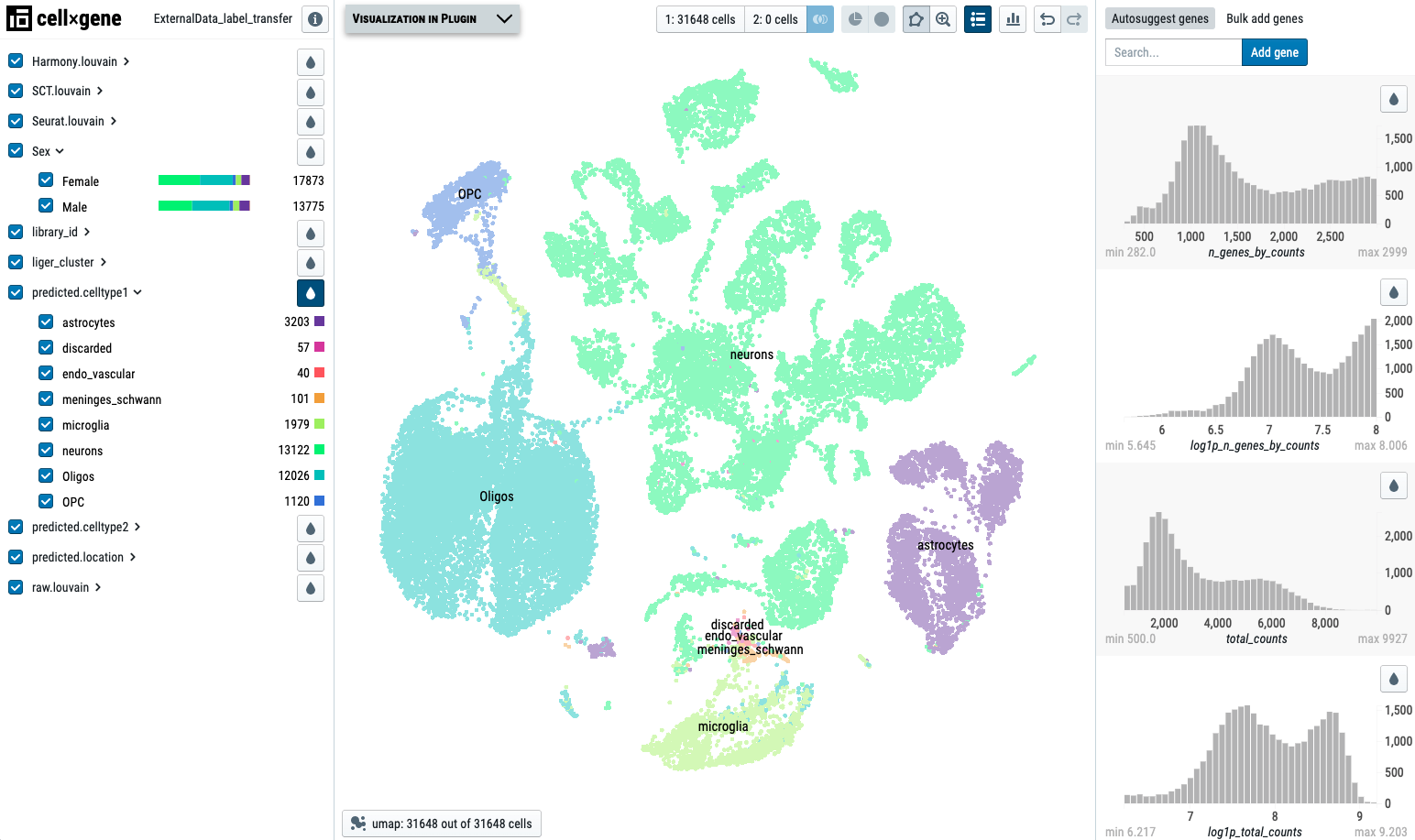
We use a UMAP with label transferred cell type annotation as an example dataset. Label transfer is strongly suggested if you would like to run DE analysis because the clusters are more meaningful than the original clusters assigned by the software:
8.1 Example 1
In the first example, we would like to run DE analysis between ‘Female’ and ‘Male’ for each cluster annotated by predicted.celltype1. In the first column, we input the header name library_id, which annotates the data sources. Then we add predicted.celltype1 in the cluster column, which allows the pipeline to loop through each cluster in predicted.celltype1. The group column contains the header name storing the comparison groups, and here we use the Sex annotation. Each time, the pipeline can only compare two conditions, such as ‘Female’ and ‘Male’. If the group column contains more groups, please list them in multiple lines in the DEGinfo.csv file.
We can also add covars if needed, but this is optional.
The default DE analysis is performed by NEBULA. As for the model, NEBULA provides two choices: HL and LN. For more details about them, please refer to the NEBULA manual.
Here is the DEGinfo.csv we described above:
comparisonName,sample,cluster,group,alt,ref,covars[+ separated],method[default NEBULA],model[default HL]
Compare_Female_vs_Male,library_id,predicted.celltype1,Sex,Female,Male,,NEBULA,HL
After preparing the DEGinfo.csv file, simply add it to the config.yml file:
DEG_desp: ~/E-MTAB-11115/processing/DEGinfo.csvThen rerun the pipeline. The pipeline won’t run the previous steps (i.e. filtering, harmonization, etc.) again, so it will directly run the DE analysis based on the harmonized h5ad file.
scAnalyzer Path/to/a/config/file

#Example:
scAnalyzer ~/E-MTAB-11115/processing/config.yml
This step may take a few hours to run. The output files will be generated in the directory:
outputdir
... previous results #Omitted, see section 6.4
├── ProjName_scDEG #Folder containing DEG results
├── Compare_Female_vs_Male
├── Female.vs.Male_predicted.celltype1:astrocytes_NEBULA.csv #Each comparison has three associated files
├── Female.vs.Male_predicted.celltype1:astrocytes_NEBULA.png
├── Female.vs.Male_predicted.celltype1:astrocytes_NEBULA.QC.pdf
├── Female.vs.Male_predicted.celltype1:discarded_NEBULA.csv
├── Female.vs.Male_predicted.celltype1:discarded_NEBULA.png
├── Female.vs.Male_predicted.celltype1:discarded_NEBULA.QC.pdf
...
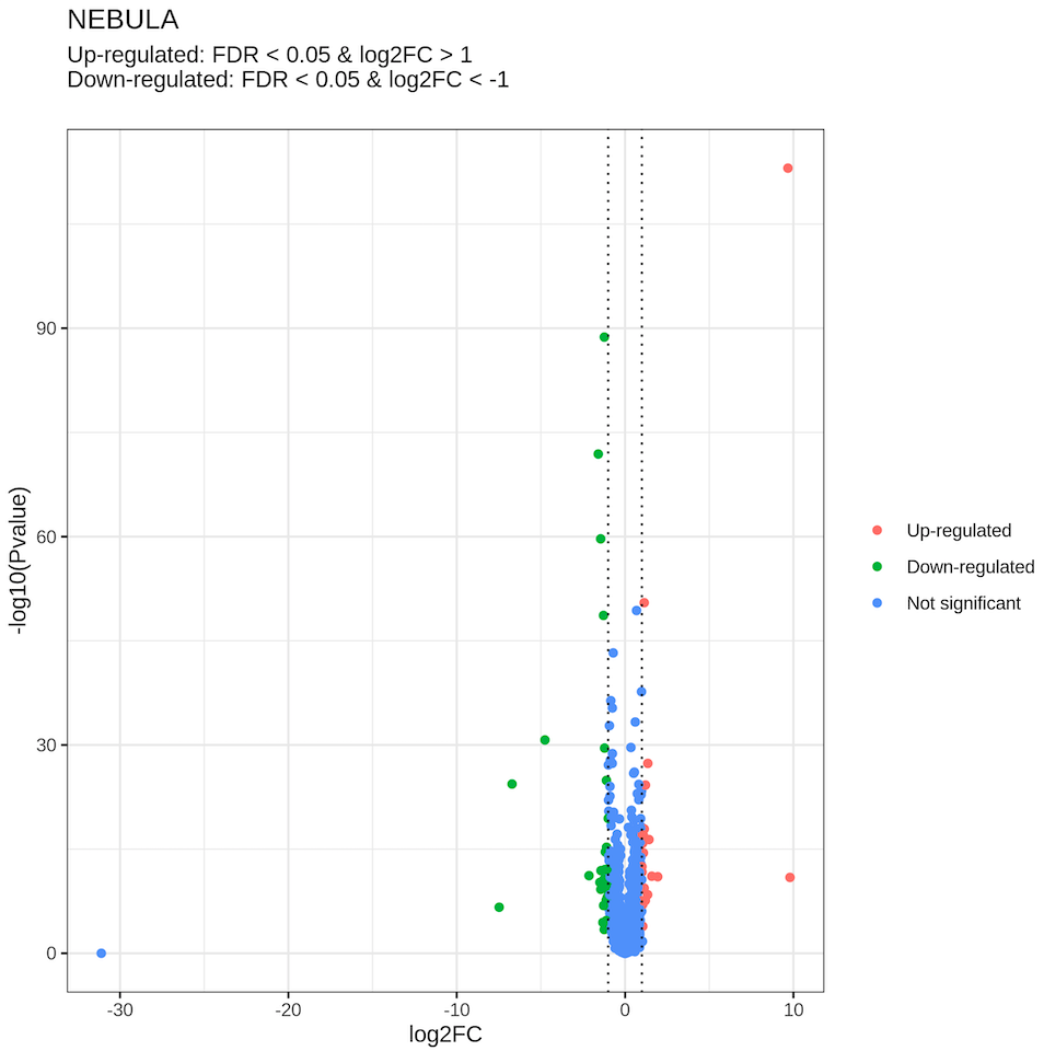
└── env.rdsAn example of the DE csv table (Female.vs.Male_predicted.celltype1/astrocytes_NEBULA.csv, top 5 rows):
In the table below, the most significant gene is Xist, a well-known X-chromosome gene highly expressed in female.
| res.tab.ID | res.tab.log2FC | res.tab.Pvalue | res.tab.FDR | res.tab.algorithm | res.tab.convergence | res.tab.metric | res.ls.summary.logFC_.Intercept. | res.ls.summary.logFC_.GrouPalt | res.ls.summary.se_.Intercept. | res.ls.summary.se_.GrouPalt | res.ls.summary.p_.Intercept. | res.ls.summary.p_.GrouPalt | res.ls.summary.gene_id | res.ls.summary.gene | res.ls.overdispersion.Subject | res.ls.overdispersion.Cell | res.ls.convergence | res.ls.algorithm |
|---|---|---|---|---|---|---|---|---|---|---|---|---|---|---|---|---|---|---|
| Xist | 9.676171 | 0 | 0 | HL | 1 | 6115.1780 | -6.693213 | 0.1276737 | 0.0234622 | 0.0469395 | 0 | 0.0065289 | 1 | Rgs20 | 0.0016728 | 0.4393152 | 1 | NBGMM (HL) |
| Pnpla7 | -1.230034 | 0 | 0 | HL | 1 | 1653.1553 | -9.321192 | -0.1694550 | 0.0534180 | 0.1065177 | 0 | 0.1116405 | 2 | Atp6v1h | 0.0064320 | 0.3327316 | 1 | NBGMM (HL) |
| Etnppl | -1.592058 | 0 | 0 | HL | 1 | 525.8328 | -8.511808 | 0.0917939 | 0.0282832 | 0.0565059 | 0 | 0.1042691 | 3 | Rb1cc1 | 0.0001000 | 0.1725113 | 1 | NBGMM (HL) |
| Zbtb16 | -1.448309 | 0 | 0 | HL | 1 | 1260.9518 | -9.896064 | -0.0918014 | 0.0584728 | 0.1165549 | 0 | 0.4309170 | 4 | 4732440D04Rik | 0.0014745 | 0.7288504 | 1 | NBGMM (HL) |
| Sorcs2 | 1.137956 | 0 | 0 | HL | 1 | 1398.0881 | -8.573613 | -0.2252848 | 0.0303869 | 0.0604625 | 0 | 0.0001945 | 5 | Pcmtd1 | 0.0001000 | 0.3502587 | -10 | NBGMM (HL) |
An example of the DE png file (Female.vs.Male_predicted.celltype1/astrocytes_NEBULA.png):
8.2 Example 2
In the second example, we are going to show how to perform DE analysis between two cell types. To achieve this, we added one artificial column (called ‘SelectAll’) in the sampleMeta.csv file, and assigned the same values (‘Everything’) to all the data:
Sample_Name,h5path,Sex,SelectAll
5705STDY8058280,/home/ysun4/testSinglecell/ExternalData/5705STDY8058280_filtered_feature_bc_matrix.h5,Female,Everything
5705STDY8058281,/home/ysun4/testSinglecell/ExternalData/5705STDY8058281_filtered_feature_bc_matrix.h5,Female,Everything
5705STDY8058282,/home/ysun4/testSinglecell/ExternalData/5705STDY8058282_filtered_feature_bc_matrix.h5,Female,Everything
5705STDY8058283,/home/ysun4/testSinglecell/ExternalData/5705STDY8058283_filtered_feature_bc_matrix.h5,Male,Everything
5705STDY8058284,/home/ysun4/testSinglecell/ExternalData/5705STDY8058284_filtered_feature_bc_matrix.h5,Male,Everything
5705STDY8058285,/home/ysun4/testSinglecell/ExternalData/5705STDY8058285_filtered_feature_bc_matrix.h5,Male,Everything
Then we prepare the DEGinfo.csv file in this way. The ‘SelectAll’ was filled into the cluster column, and since it only has one value, it actually selects all cells when running the pipeline. Then it performs astrocytes to Oligos comparison.
comparisonName,sample,cluster,group,alt,ref,covars[+ separated],method[default NEBULA],model[default HL]
Comparison_Ast_vs_Oligo,library_id,SelectAll,predicted.celltype1,astrocytes,Oligos,,NEBULA,HL
Then we need to run the scRNASequest pipeline from the beginning, which allows the ‘SelectAll’ column to be embedded into the harmonized h5ad output. As long as we have DEGinfo.csv included in the config.yml, it will run through the DE analysis and produce the following results:
outputdir
... previous results #Omitted, see section 6.4
├── ProjName_scDEG #Folder containing DEG results
├── Comparison_Ast_vs_Oligo
├── astrocytes.vs.Oligos_SelectAll:Everything_NEBULA.csv #Each comparison has three associated files
├── astrocytes.vs.Oligos_SelectAll:Everything_NEBULA.png
├── astrocytes.vs.Oligos_SelectAll:Everything_NEBULA.QC.pdf
├── env.rds
├── ProjName_scDEG.cmd.json
├── deg6602_SelectAll_predicted.celltype1_NEBULA_HL_Everything_astrocytes_Oligos.error #Standard error messages
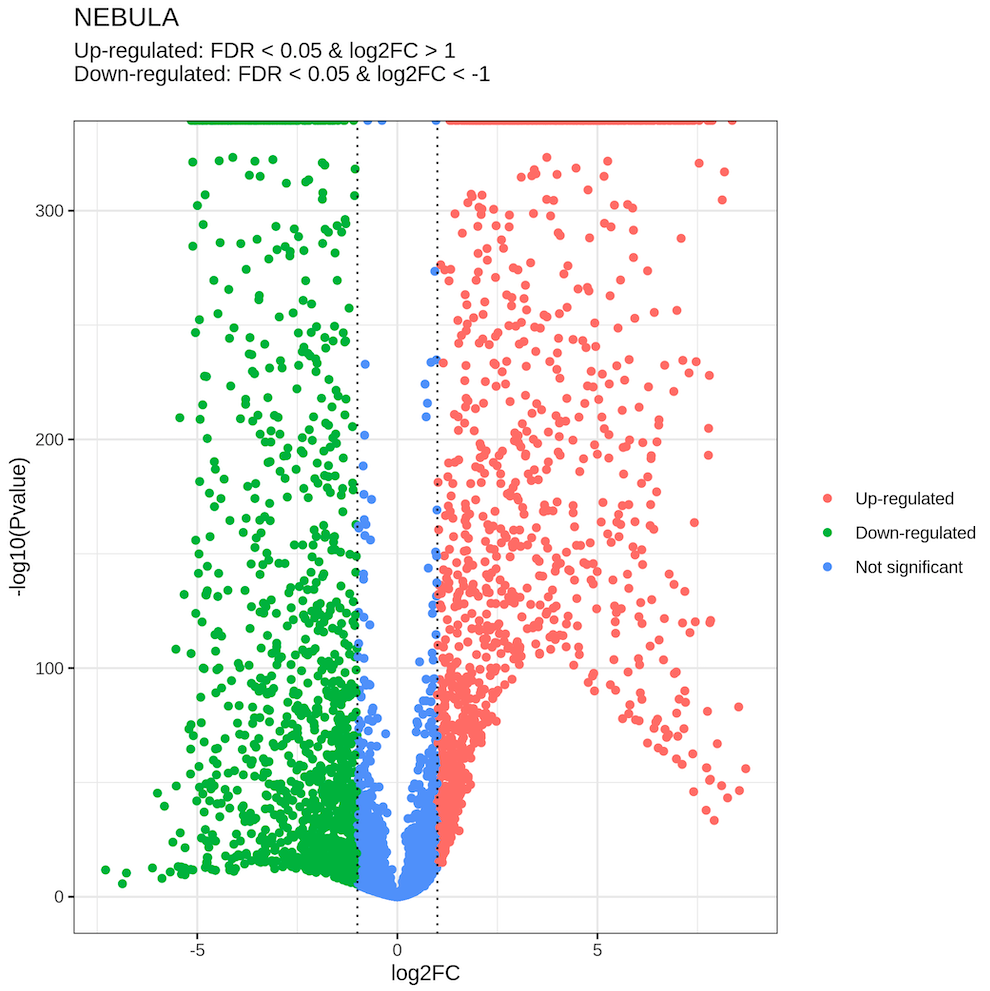
└── ProjName_scDEG.dbAn example of the DE csv table (astrocytes.vs.Oligos_SelectAll:Everything_NEBULA.csv, top 5 rows):
| res.tab.ID | res.tab.log2FC | res.tab.Pvalue | res.tab.FDR | res.tab.algorithm | res.tab.convergence | res.tab.metric | res.ls.summary.logFC_.Intercept. | res.ls.summary.logFC_.GrouPalt | res.ls.summary.se_.Intercept. | res.ls.summary.se_.GrouPalt | res.ls.summary.p_.Intercept. | res.ls.summary.p_.GrouPalt | res.ls.summary.gene_id | res.ls.summary.gene | res.ls.overdispersion.Subject | res.ls.overdispersion.Cell | res.ls.convergence | res.ls.algorithm |
|---|---|---|---|---|---|---|---|---|---|---|---|---|---|---|---|---|---|---|
| Xkr4 | -3.327923 | 0 | 0 | HL | 1 | 4177.156 | -8.168075 | -2.3067403 | 0.0367924 | 0.0561022 | 0 | 0.0000000 | 1 | Xkr4 | 0.0067297 | 0.6076303 | 1 | NBGMM (HL) |
| Rgs20 | 6.386205 | 0 | 0 | HL | 1 | 5561.771 | -9.825703 | -2.5066029 | 0.0890548 | 0.1353916 | 0 | 0.0000000 | 2 | Gm1992 | 0.0398103 | 1.4947561 | 1 | NBGMM (HL) |
| St18 | -5.129500 | 0 | 0 | HL | 1 | 14283.487 | -10.322696 | 0.2176484 | 0.0310922 | 0.0690489 | 0 | 0.0016211 | 3 | Mrpl15 | 0.0001000 | 0.4188721 | 1 | NBGMM (HL) |
| Adhfe1 | 4.842192 | 0 | 0 | HL | 1 | 12162.136 | -10.169996 | 0.1119117 | 0.0292679 | 0.0669762 | 0 | 0.0947381 | 4 | Tcea1 | 0.0001000 | 0.7212448 | 1 | NBGMM (HL) |
| Prex2 | 8.368190 | 0 | 0 | HL | 1 | 8249.837 | -10.292221 | 4.4265797 | 0.0513462 | 0.0563860 | 0 | 0.0000000 | 5 | Rgs20 | 0.0047768 | 0.4563594 | 1 | NBGMM (HL) |
An example of the DE png file (astrocytes.vs.Oligos_SelectAll:Everything_NEBULA.png):
8.3 Example 3
In this example, we show how to perform DE analysis using multiple software. In the config file, each line is a comparison, and for the same comparison (treat v.s. control), we can set up multiple runs using different DE tools as below:
comparisonName,sample,cluster,group,alt,ref,covars[+ separated],method[default NEBULA],model[default HL]
Treated_vs_Control_nebula,library_id,sctHarmony_cluster_predicted.celltype,Treatment,Treated,Vehicle,,NEBULA,HL
Treated_vs_Control_t_test,library_id,sctHarmony_cluster_predicted.celltype,Treatment,Treated,Vehicle,,t_test,
Treated_vs_Control_u_test,library_id,sctHarmony_cluster_predicted.celltype,Treatment,Treated,Vehicle,,u_test,
Treated_vs_Control_edgeR,library_id,sctHarmony_cluster_predicted.celltype,Treatment,Treated,Vehicle,,edgeR,
Treated_vs_Control_limma,library_id,sctHarmony_cluster_predicted.celltype,Treatment,Treated,Vehicle,,limma,
Treated_vs_Control_DESeq2,library_id,sctHarmony_cluster_predicted.celltype,Treatment,Treated,Vehicle,,DESeq2,
Treated_vs_Control_MAST,library_id,sctHarmony_cluster_predicted.celltype,Treatment,Treated,Vehicle,,MAST,
Treated_vs_Control_limma_cell_level,library_id,sctHarmony_cluster_predicted.celltype,Treatment,Treated,Vehicle,,limma_cell_level,
Treated_vs_Control_glmmTMB,library_id,sctHarmony_cluster_predicted.celltype,Treatment,Treated,Vehicle,,glmmTMB,poisson
Treated_vs_Control_ancova,library_id,sctHarmony_cluster_predicted.celltype,Treatment,Treated,Vehicle,,ancova,
Please note that NEBULA and glmmTMB require model information.
For NEBULA, users can choose from HL and LN, and the pipeline uses ‘HL’ by default. The differences between them can be found in the NEBULA GitHub page:
“NEBULA-LN is faster and performs particularly well when the number of cells per subject (CPS) is large. In addition, NEBULA-LN is much more accurate in estimating a very large subject-level overdispersion. In contrast, NEBULA-HL is slower but more accurate in estimating the cell-level overdispersion.”
For glmmTMB, it is required to choose a model from the following: “nbinom2”, “nbinom1”, “poisson”, “nbinom2zi”, “nbinom1zi”.