Chapter 6 Advanced Analyses

6.1 Correlation Tools

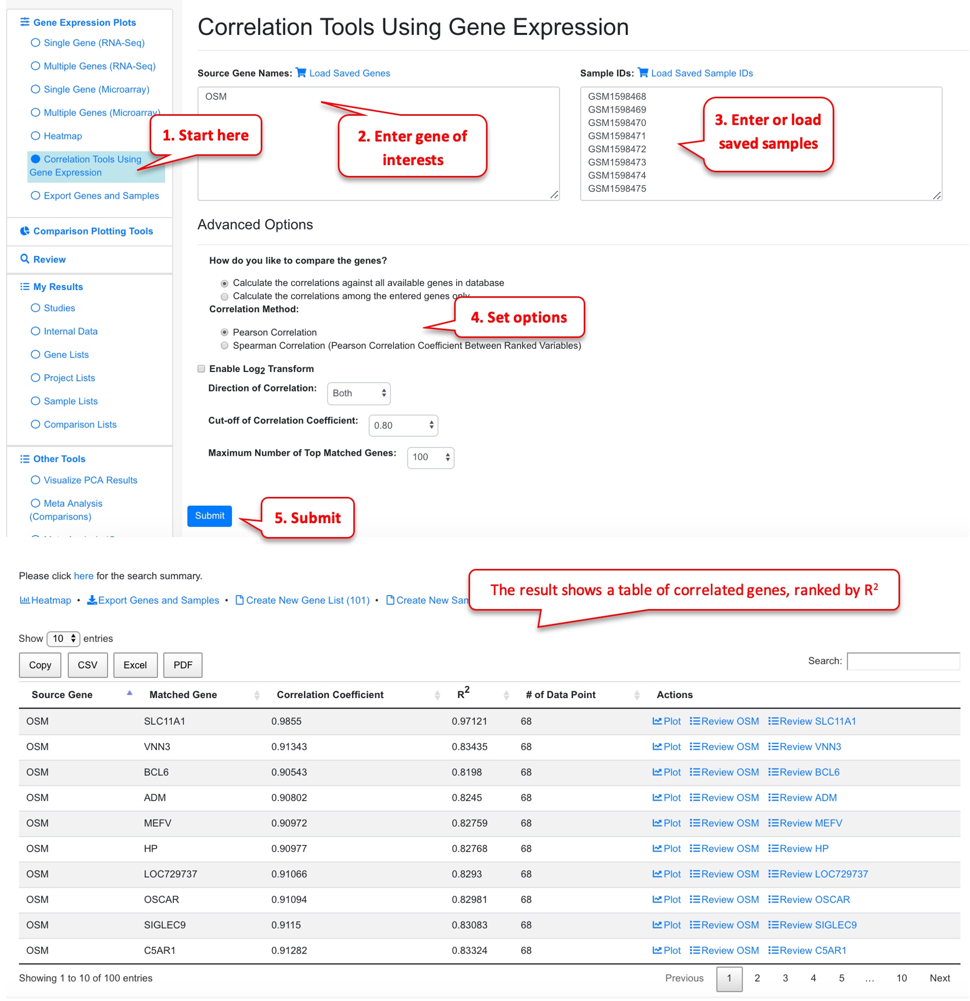
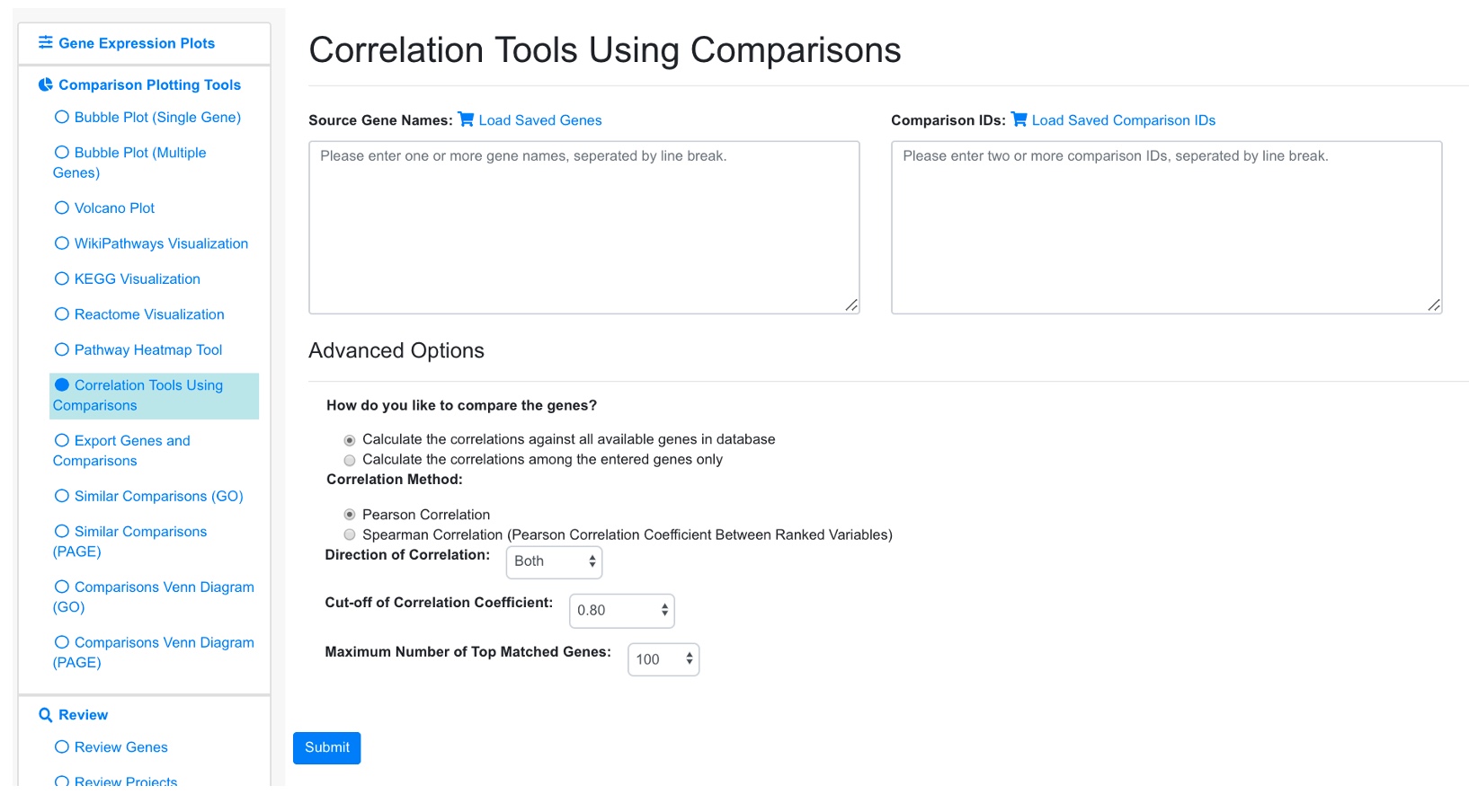
Once the user has identified a gene of interest, the user can use correlation tools to find other genes that share similar (or opposite) profiles in terms of gene expression or fold change. First, enter the gene of interest, and samples to be used for correlation. In the example below, we entered OSM gene, and 69 samples involved in Crohn’s disease.

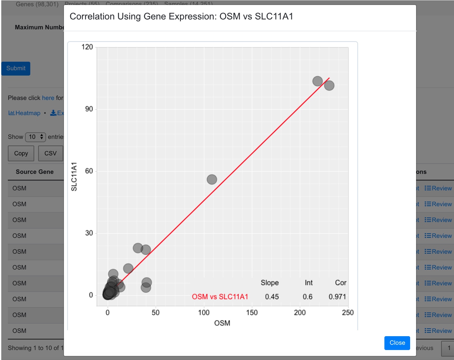
Click the plot icon will show scatter plot of the target and the correlated gene.

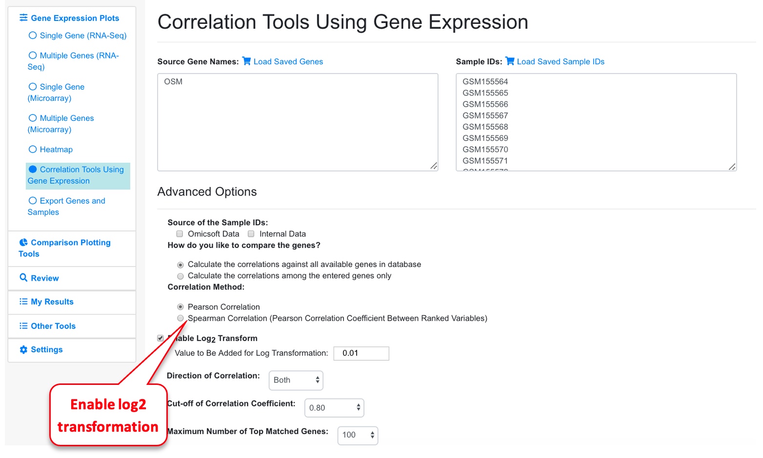
An additional way to plotting the correlation with other genes, is to enable the log2 transformation of the expression.

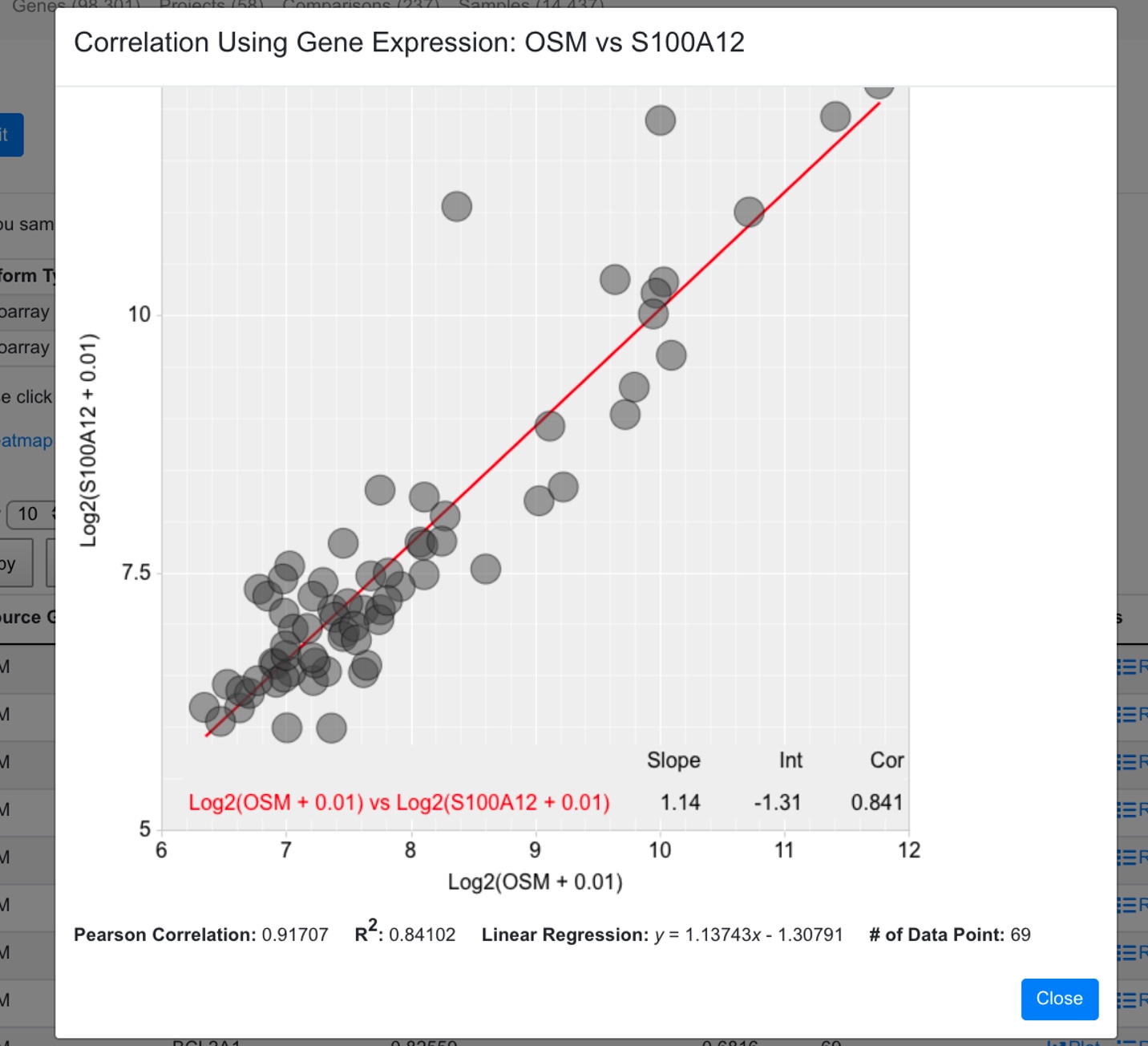
Now the expression is log transformed.

The examples above are from Correlation Tools using Expression. The interface and usage for Correlation Tools using Comparison is similar.

6.2 PCA Analysis

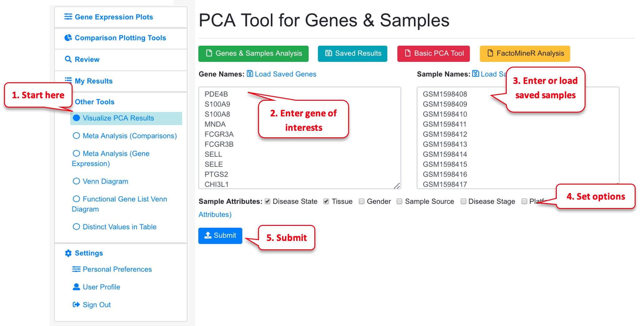
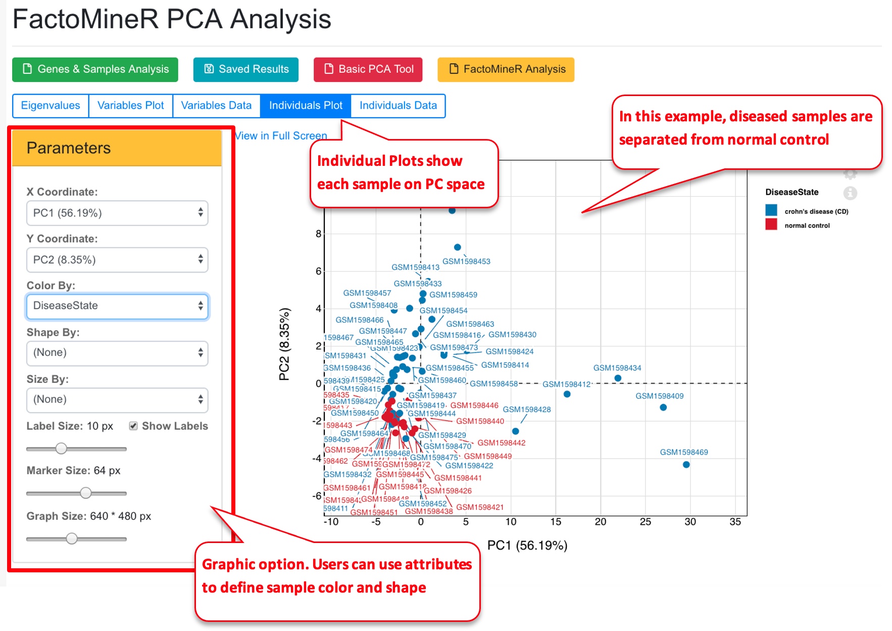
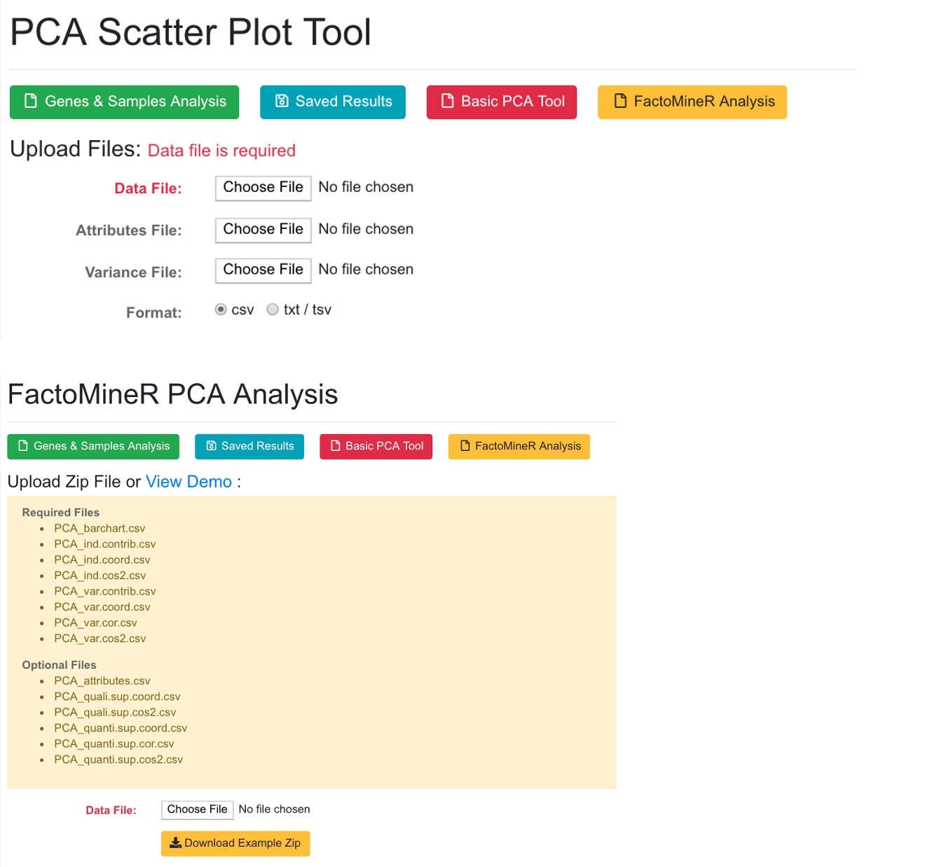
Users can select a few samples and use PCA plot to visualize the sample relationships.

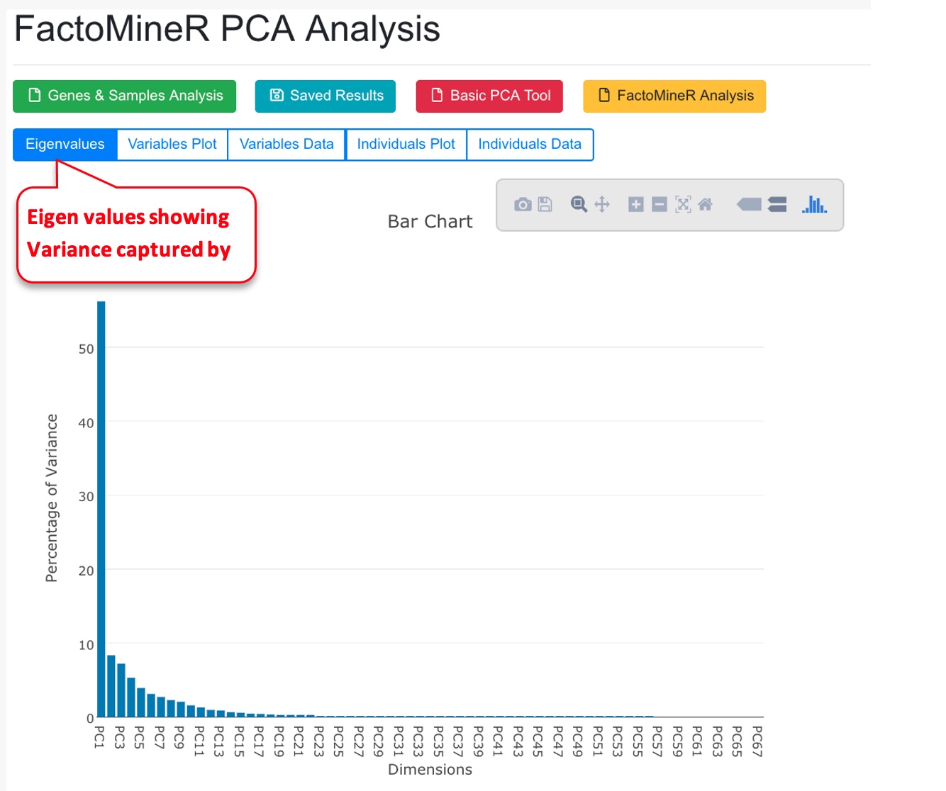
The system will use FactorMineR package to run PCA analysis and display the results.

The PCA tool can also display results from pre-calculated data (basic PCA, or FactorMineR results).

6.3 Meta-Analysis

Meta-Analysis can be used to identify genes that are changed consistently across multiple projects. This can be either implemented by doing Meta-analysis using comparisons or meta-analysis using gene expression.

6.3.1 Meta-Analysis (Comparisons)

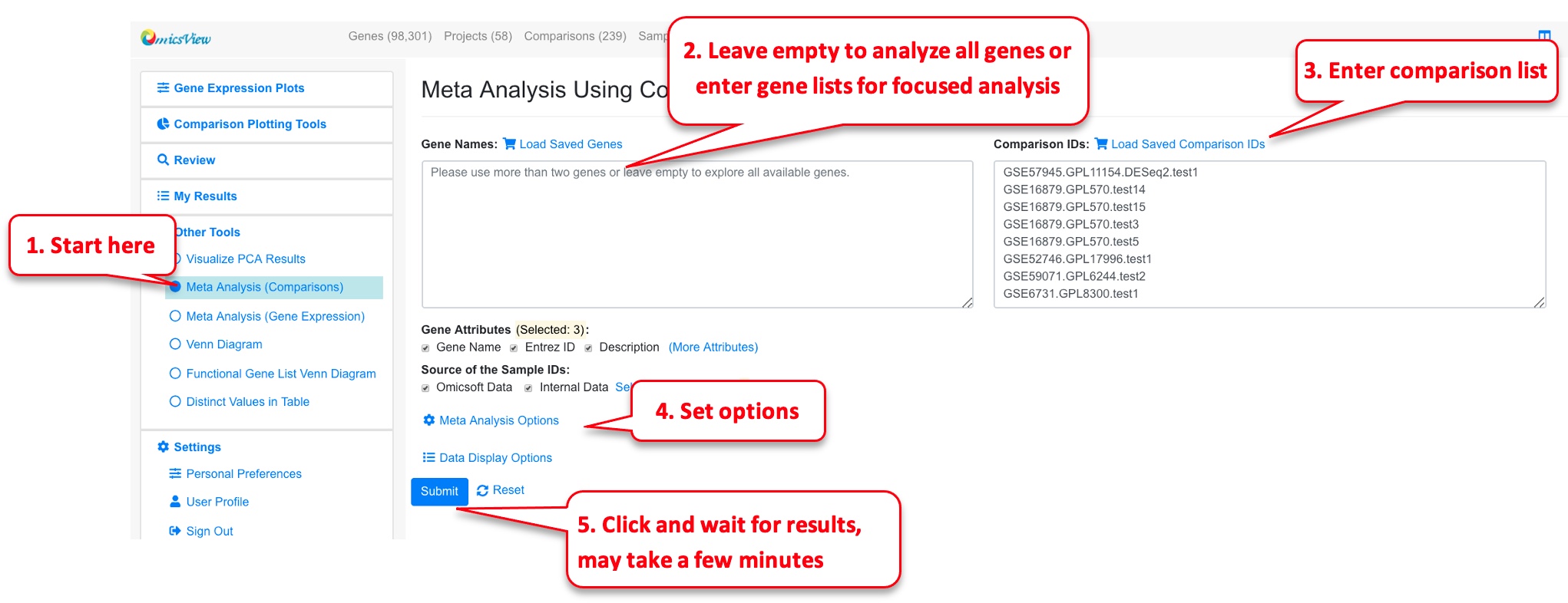
In the example below, we are looking for the most significant DEGs in Disease vs. Normal comparisons of Crohn’s Disease.

The system will use the comparison data (logFC, p-value) to compute combined p-value and rank product. It also uses a simple cutoff to get counts of up and down-regulated genes. This method is fast and can be applied to any comparison data. However, it does not use the individual sample data or consider number of samples in each comparison.

We can enable filter by percentage up-regulated genes to focus on genes that are consistently up-regulated.

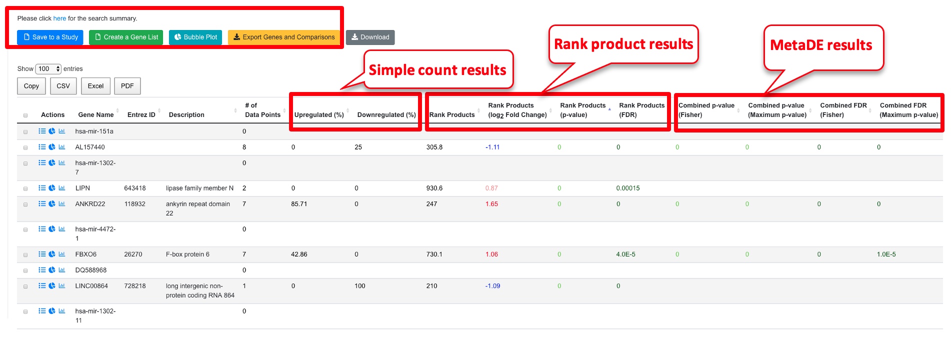
From the output table, the user can select the genes most interesting to them. Some key columns are explained below.

• # of data points: this shows the number of comparisons with valid data for this gene. Although 8 comparisons were entered here, not all genes show up in all experiments. We used minimal 3 data points when we set up display options.
• Simple count results. Using the cutoff values we entered (logFC 1, FDR 0.05), the system checks if a gene passes the cutoff for each comparison, and computes percentage up and down regulation.
• Rank Product results (recommended results for meta-analysis). This is done with the RankProd package. The system ranks genes in each comparison using logFC and computes a combined rank and statistical values. The Rank Products columns show the rank (smaller is more consistent change), log2Fold Change and FDR.
• The Combined p-value/FDR (Fisher or Maximum) are computed using the individual p-values with MetaDE package. Note unlike RankProd, these values didn’t consider the direction of the change, so the data need to be interpreted carefully, and we recommend using these p-values together with the simple count values to have a better understanding.

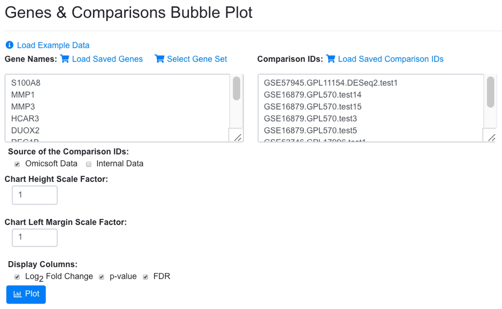
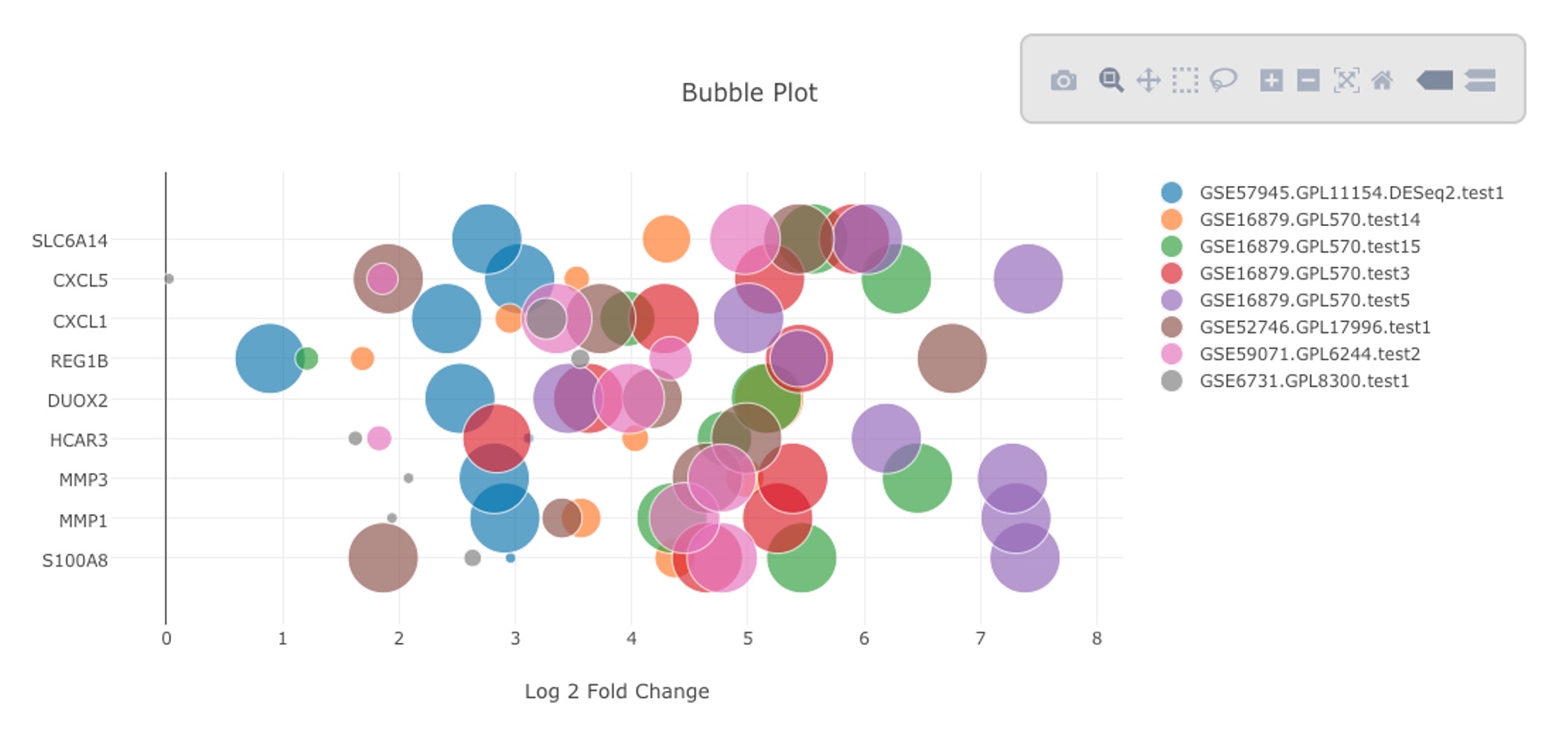
The table can be sorted by any column. In the above view, we sorted the data by logFC. The table can also be sorted by # of data points to view the genes with most data. In the example below, we chose 10 up-regulated genes with most data points form the table and used the bubble plot button to create bubble plot. It can be seen that indeed all these genes show consistent up-regulated in the selected comparisons.

The resulting bubble plot will show all 8 comparisons for each gene.

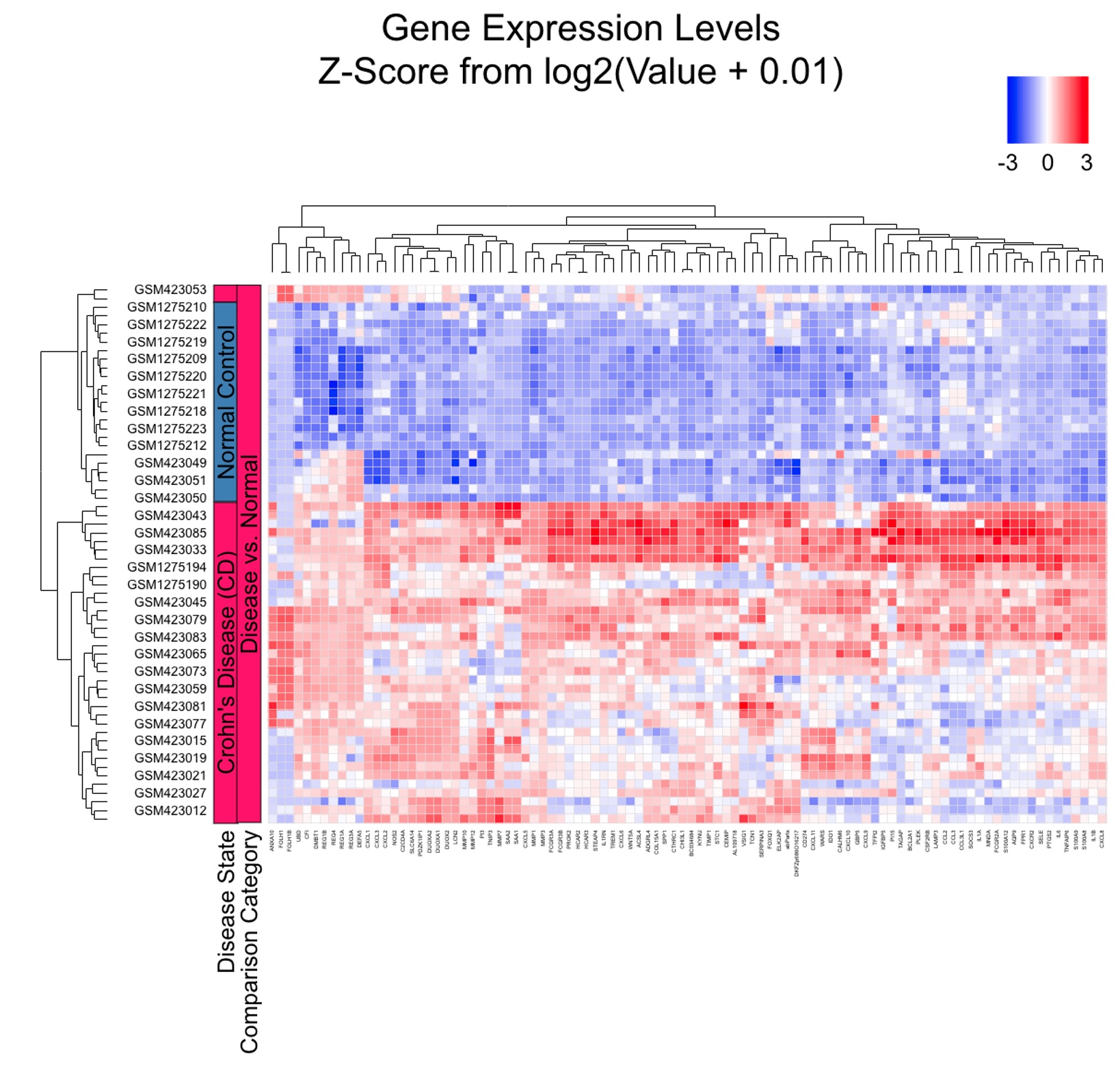
We can also create a gene list from the table for up or down gene lists from meta-analysis (using the green button at top of meta-analysis results) and use the list for subsequent analysis like functional enrichment or generating heatmap. Below is a heatmap using 100 up-regulated genes from meta-analysis, and it is very clear that the diseased samples have an upregulation of these genes.

6.3.2 Meta-Analysis (Gene Expression)

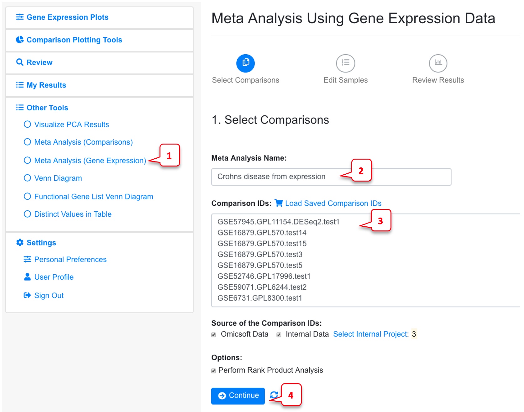
In the example below, we use the same comparisons from Crohn’s disease.

By default, the Rank Product Analysis is checked. Uncheck this if the data is too big for Rank product analysis, or you just need a quick run using limma for each individual comparison.

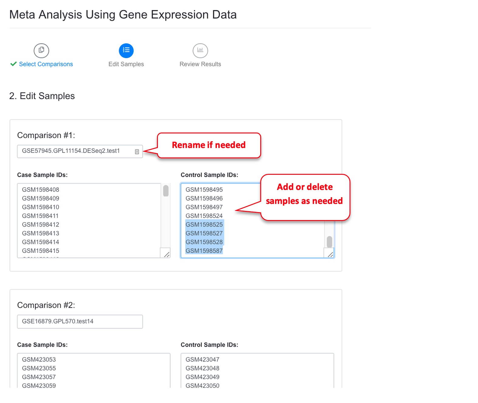
On the next page, system will display the Case and Control samples for each comparison. At this step, users can edit samples. Users can use this page to remove outliers or add other samples they want to include in the meta-analysis.

After users review the samples for each comparison, they can go to the next step to run the meta-analysis. This step can take a while if the number of samples is large. For the meta-analysis, the system will do the following:

1. Run limma to get logFC, p-value and confidence interval for each individual comparison

2. Run MetaDE to get combined p-values

3. Run Rank Product package for all the expression data to get statistical significance and combined logFC.

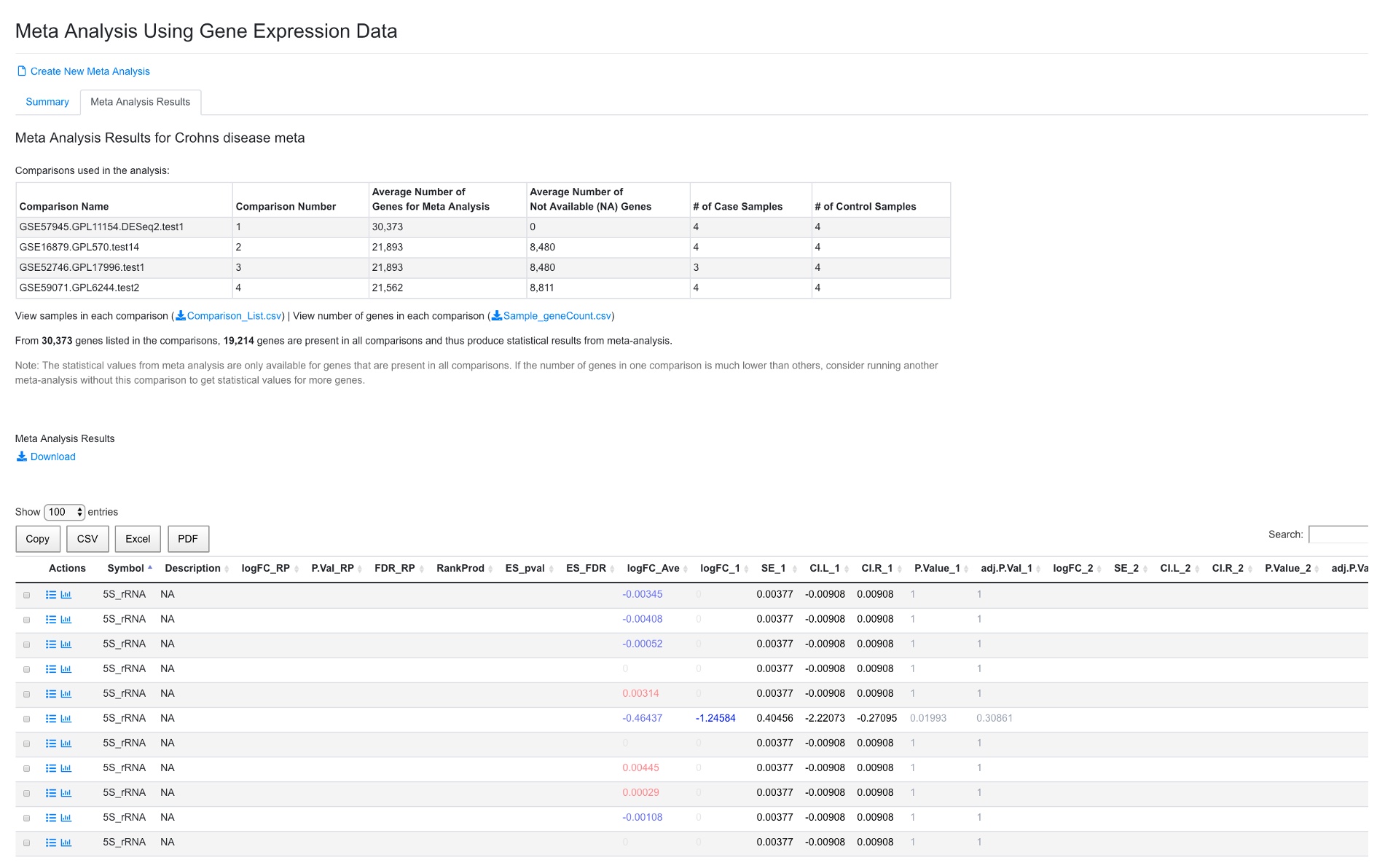
After the analysis is done, the system will show a summary and the result table.

In the summary, the four comparisons are shown, along with number of genes used for meta-analysis, and number of case and control samples. Because different platforms (especially arrays) have different number of genes present, and some genes may have too low signals to be detected in certain projects, not all genes are present in all the comparisons. In this example, 19,214 genes are present in all comparisons. In some cases, it may be beneficial to remove some comparisons with small number of genes.

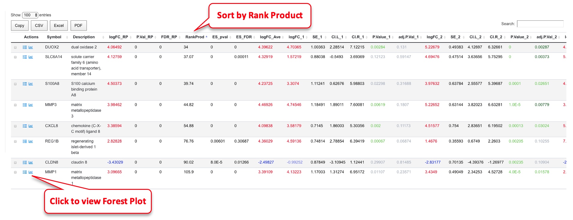
In the meta-analysis result table, results from Rank Product are shown (from RankProd package, preferred results to use), followed by effective size method (MetaDE.ES from MetaDE package). The logFC, SE, confidence interval, p-value and FDR for each comparison are shown next. The comparison numbers are the same as those listed in the summary table above. The gene list can be sorted by RankProd (most significant changes) or by logFC_RP (up or down-regulated).

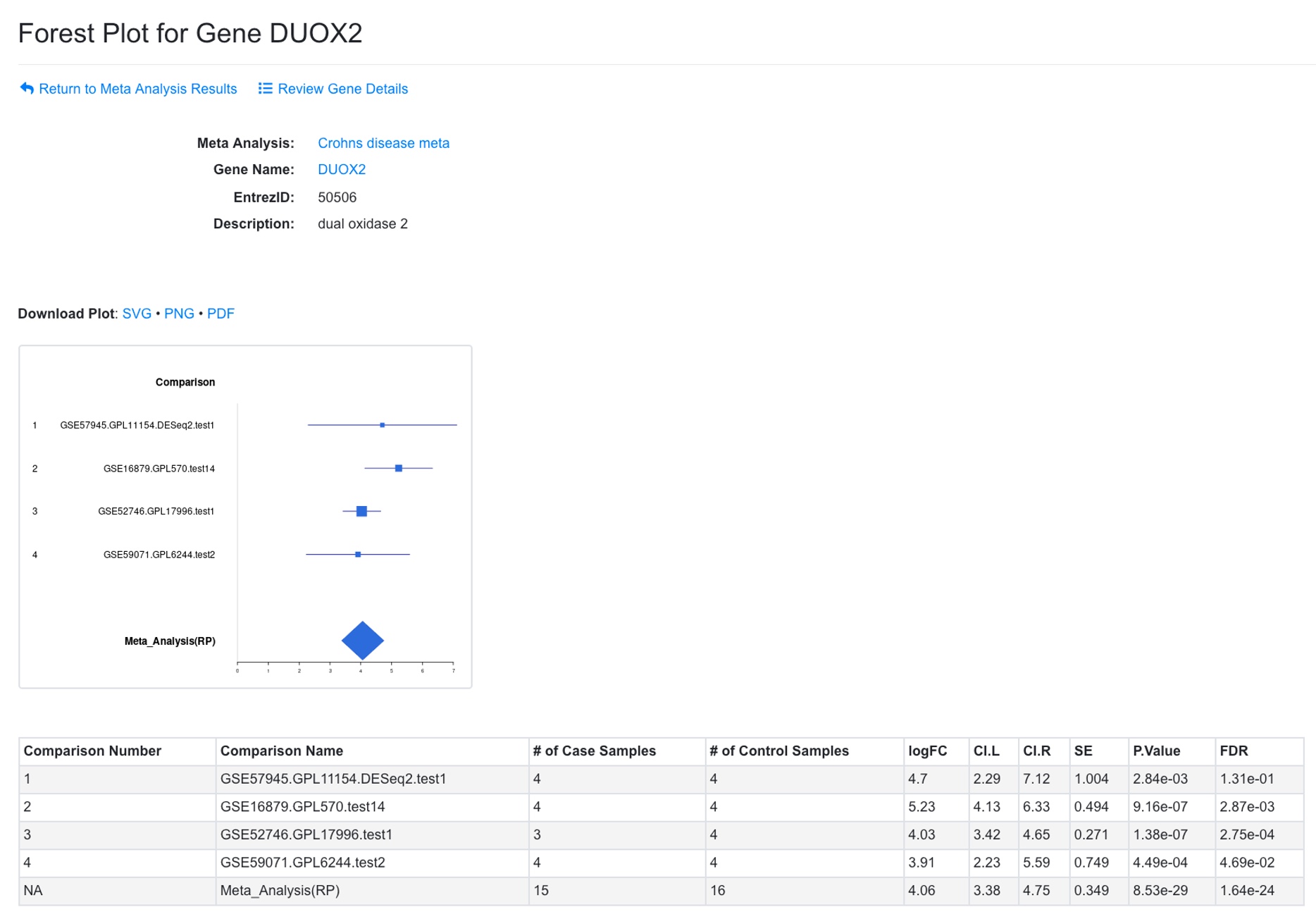
From this analysis, we can create a Forest plot for each gene by clicking the icon near the gene symbol.

In the Forest plot, results from individual comparison and combined data are shown. The confidence interval for individual comparison is based on limma output. The confidence interval for combined results is based on p-value from RankProd (or ES method when RankProd is not run).

The plot can be saved as SVG or PDF. The summary table is shown below the plot.