Chapter 7 GeoMX

GeoMx™ Digital Spatial Profiler (DSP) is a spatial transcriptomics platform developed by NanoString Technologies (Now Bruker Corporation), allowing researchers to quantify RNA and/or protein expression using FFPE (formalin-fixed, paraffin-embedded) or fresh frozen samples. GeoMx enables high-plex, spatially resolved profiling of tissues based on user-defined Region of interests (ROIs). These ROIs can be defined using multiple staining markers, and each ROI usually has at least 50–100 cells, but ideally 100–300+ cells per ROI for robust RNA signal. Thus, GeoMx cannot provide single-cell resolution spatial transcriptomics readout, but it allows better capture of lowly-expressed genes, due to its mini-bulk strategy.

GeoMx experiment can be sequenced using NGS high-throughput sequencing, or counted using NanoString nCounter. Here, we discuss the data analysis using NGS-based readout, with DCC as pipeline input format.

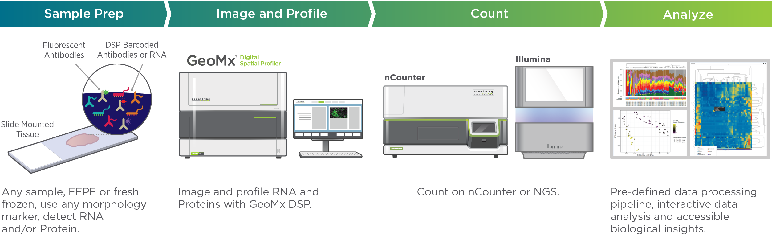
GeoMx workflow: This figures shows the general workflow of GeoMx experiment. The whole workflow contains sample preparation, imaging, data collection, and downstream data analysis. (Image from: https://nanostring.com/products/geomx-digital-spatial-profiler/geomx-dsp-overview/)

7.1 FASTQ to DCC conversion

NanoString Technologies (Now Bruker Corporation) provides a toolkit to process GeoMx readout in the FASTQ format. As described here, users can follow the instruction and generate files with .dcc as suffix for downstream analysis.

Another useful user manual is available at: GeoMx DSP NGS Readout User Manual

7.2 Pipeline setup

Demo run directory: ~/SpaceSequest_demo/4_GeoMx

Here, we will demonstrate the pipeline using a public dataset provided by NanoString Technologies. The FASTQ->DCC step has already been run for this data, so we can directly start from DCC file processing.

The demo dataset is a public data provided by NanoString: http://nanostring-public-share.s3-website-us-west-2.amazonaws.com/GeoScriptHub/Kidney_Dataset_for_GeomxTools.zip. After unzipping this file, please add the following file to the annotation folder inside Kidney_Dataset, as we modified the spreadsheet to simplify this test run: https://github.com/interactivereport/SpaceSequest/blob/gh-pages/tutorial/02-Introduction.Rmd

This is a kidney dataset, and in our demo run, we will run data processing, quality control, and differential expression analysis by comparing two kidney cell types: Glomerulus v.s. Tubule

First, we initiate the pipeline using the following script. This will generate templates of config.yml and compareInfo.csv:

#First step, generate config and sampleMeta file

geomx ~/SpaceSequest_demo/4_GeoMx

After this step, fill in the config.yml file and the sampleMeta.csv file as below:

#config file for GeoMx. Please avoid using spaces in names or paths. All items are required.

project_ID: GeoMx_demo                                        #name of the project

data_path: ~/SpaceSequest_demo/4_GeoMx/Kidney_Dataset/dccs    #path to DCC files

data_annotation: ~/SpaceSequest_demo/4_GeoMx/Kidney_Dataset/annotation/kidney_demo_AOI_Annotations_selected_clean.xlsx        #sample meta information

annotation_sheet: Template                                    #Sheet name of annotation Excel file

pkcs_file: ~/SpaceSequest_demo/4_GeoMx/Kidney_Dataset/pkcs/TAP_H_WTA_v1.0.pkc       #path to the pkc file

output_dir: ~/SpaceSequest_demo/4_GeoMx/results               #path for output files

comparison: ~/SpaceSequest_demo/4_GeoMx/compareInfo.csv       #comparison file to define DE groups

quickomics: True

Then prepare the compareInfo.csv file to define differential expression analysis comparisons:

CompareName,Model,Group_name,Group_test,Group_ctrl,Analysis_method

Glome_vs_Tubule,~region,region,glomerulus,tubule,Linear

Currently, users can run a single linear model to call the differentially expressed genes using Q3 normalized data.

Run the pipeline as below:

#Run the data

geomx ~/SpaceSequest_demo/4_GeoMx/config.yml

Finally check the results in the output_dir folder specified in the config.yml file. The output files contain DE analysis results, and if the quickomics parameter was set to True, it will generate multiple .csv files to create a Quickomics visualization link. An example can be found here (Q3 normalized values were used to create the link): http://compbio.biogen.com:3838/Quickomics/?unlisted=PRJ_GeoMx_demo_Ij4YyG

7.3 Results

This test run only has a simple comparison so should only take a few minutes to run.

The output files are a set of .csv files containing gene expression and differential expression analysis results. These files are fully compatible with Quickomics, an R Shiny application for data exploration. Users can upload these csv files to Quickomics for downstream analysis and figure generation.

Results in the directory:

~/SpaceSequest_demo/4_GeoMx/results
  ├── Comparison_result_1.txt     #Differential expression result
  
  #Quickomics files:
  GeoMx_demo_Sample_metadata.csv
  GeoMx_demo_Exp_Q3NormData.csv
  GeoMx_demo_Comparison_Data.csv
  GeoMx_demo_ProteinGeneName_Optional.csv
  
  #Additional normalizations:
  GeoMx_demo_Exp_NegNormData.csv
  GeoMx_demo_Exp_QuantileNormData.csv

NanoString Technologies (Now Bruker Corporation) suggests using Q3 normalization, which was performed using:

demoData <- normalize(demoData ,
                             norm_method = "quant", 
                             desiredQuantile = .75,
                             toElt = "q_norm")

However, additional normalization is also available, and users can upload those normalized values to Quickomics for analysis. For example, the ‘Negative Probe’ normalization was performed by the following command:

target_demoData <- normalize(target_demoData ,
                             norm_method = "neg", 
                             fromElt = "exprs",
                             toElt = "neg_norm")

7.4 Quickomics exploration

Here, we upload the following four files to the Quickomics server:

GeoMx_demo_Sample_metadata.csv: Sample meta information include sameple name, disease conditions, etc.
GeoMx_demo_Exp_Q3NormData.csv: Gene expression values normalized by Q3 normalization
GeoMx_demo_Comparison_Data.csv: Differential expression analysis results
GeoMx_demo_ProteinGeneName_Optional.csv: Gene-Protein name conversion

Quickomics link: https://quickomics.bxgenomics.com/?unlisted=PRJ_GeoMx_demo_238wZk

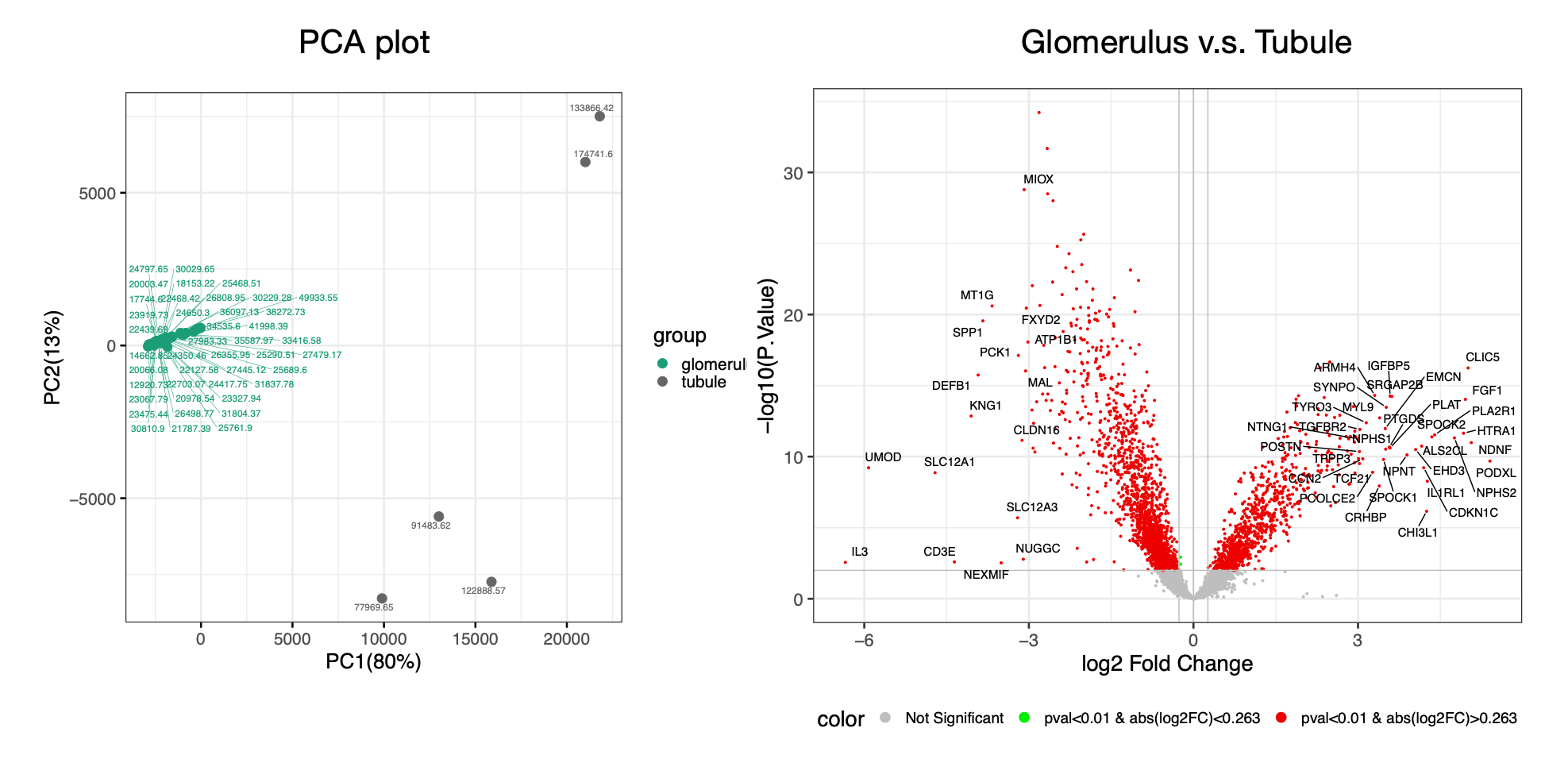
A few example images from Quickomics exploration. The figure below shows GeoMx PCA and volcano plots:

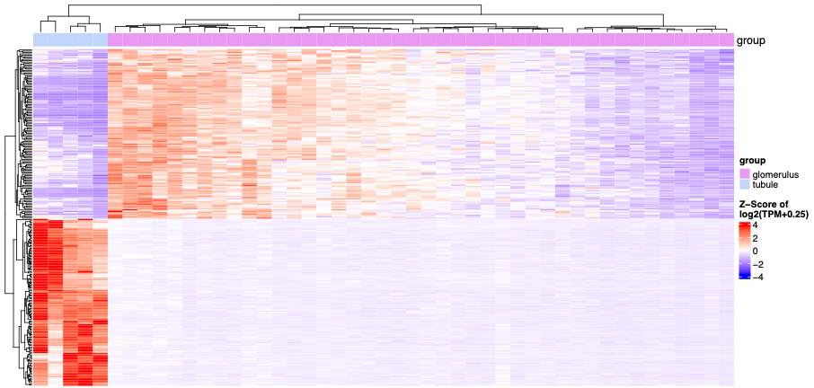
The following figure displays a GeoMx expression heatmap: