Chapter 9 Additional tools
In this section, we introduce three additional tools to further analyze spatial transcriptomics data.
9.1 cosMx2VIP
We have introduced previously that NanoString CosMx data can be analyzed through SpaceSequest cosmx workflow. However, the cosmx workflow does not incorporate the original images for visualization. Here, we developed another tool, called cosMx2VIP, to add CosMx images to the gene expression data, creating an integrated object, which can be further visualized by Cellxgene VIP. Cellxgene VIP not only hosts single-cell RNA-seq datasets, it also loads spatial transcriptomics data and displays the image and data simultaneously. Here, we will go through the process step-by-step.
9.1.1 Input file set up
In this section, we will go through input files that are necessary for running the cosMx2VIP workflow.
Here, we use the public CosMx dataset from NanoString website again:
Human frontal cortex FFPE data is available through: https://nanostring.com/products/cosmx-spatial-molecular-imager/ffpe-dataset/human-frontal-cortex-ffpe-dataset/
Since cosMx2VIP integrates the data and the image, it requires the images as well. Thus, we will need to download both Basic Data Files and Raw Data Export. The Basic Data Files will be a .zip file with ~15 Gb, while the Raw Data Export contains a large RawFiles.zip file with ~602 Gb. Please make sure you have enough space to store those files.
Unzipping the RawFiles.zip file resulted in the following folders. Also attached the S3 folder unzipped from Basic Data Files:
~/SpaceSequest_demo/6_cosMx2VIP/
  ├── S3/
  # S3 data files
    ├── S3_exprMat_file.csv
    ├── S3_fov_positions_file.csv
    ├── S3_metadata_file.csv
    ├── S3-polygons.csv
    ├── S3_fov_path.csv      #This file is not downloaded from the NanoString website. See below for more details to create this file.
    └── S3_tx_file.csv

  # More folders in the RawFiles.zip:
  ├── CellStatsDir/
    ├── CellComposite/
    ├── CellOverlay/
    ├── FOV001/
    ├── FOV002/
    ├── ...
    ├── FOV392/
    ├── Morphology2D/
    ├── Morphology3D/
    └── RnD/
  ├── RunB1324_S3_c_v6/
    ├── FOV001/
    ├── FOV002/
    ├── ...
    └── FOV392/
  └── RunSummary/
    ├── FovTracking/
    ├── Shading/
    ├── Affine_Transform_20220928.csv
    ├── c902.fovs.csv
    ├── latest.af.fovs.csv
    ├── latest.fovs.csv
    ├── Morphology_ChannelID_Dictionary.txt
    ├── MR-Tissue - All Channels.mkit
    ├── RunRunB1324_20230504_231244_S3_Beta04_ExptConfig.txt
    ├── RunRunB1324_20230504_231244_S3_Beta04_SpatialBC_Metrics4D.csv
    └── temp.devapptemp
Another critical file for cosMx2VIP to run is the S3_fov_path.csv file. This file is not provided by NanoString, and needs to be set up manually. It provides the directory of each fov as well as the associated image file location fov_img. ‘…’ indicates the omitted lines for simplification:
fov,fov_img
1,/SpaceSequest_demo/6_cosMx2VIP/CellStatsDir/FOV001/CellLabels_F001.tif
2,/SpaceSequest_demo/6_cosMx2VIP/CellStatsDir/FOV002/CellLabels_F002.tif
...
392,/SpaceSequest_demo/6_cosMx2VIP/CellStatsDir/FOV001/CellLabels_F392.tif
9.1.2 Run the workflow
The first step is to run the script with a path to the working directory:
cosMx2VIP ~/SpaceSequest_demo/6_cosMx2VIP/This will generate the following config.yml. Users can fill in the file using the example below:
## Please modify "required" section
prj_name: CosMx2VIP_demo                                                  # the name of the project which will be used as prefix of all file created
output: ~/SpaceSequest_demo/6_cosMx2VIP/
expression_file: ~/SpaceSequest_demo/6_cosMx2VIP/S3/S3_exprMat_file.csv   # the path to the expression file for all FOV of a capture
meta_file: ~/SpaceSequest_demo/6_cosMx2VIP/S3/S3_metadata_file.csv        # the path to the meta file for all FOV of a capture
cell_polygon_file: ~/SpaceSequest_demo/6_cosMx2VIP/S3/S3-polygons.csv     # the path to the cell polygon file for all FOV of a capture
transcript_loc_file: ~/SpaceSequest_demo/6_cosMx2VIP/S3/S3_tx_file.csv    # the path to the transcript location file for all FOV of a capture
fov_image_file: ~/SpaceSequest_demo/6_cosMx2VIP/S3/S3_fov_path.csv        # the file path to the csv link the meta FOV column to image file path,
                                                                          #    two columns: first column is the FOV identifier the same as meta file (same column header);
                                                                          #    the second ("fov_img") is the file path to the FOV image
cell_id_col: [cell_ID,cellID]                                             # the column header (first one in order) of cell ID in all data across files defined in above sample_meta
suffix_local_px: _local_px                                                # the suffix of pix location in one capture image, such that x coordinates column header is regular expression ".*x.*_local_px"
suffix_global_px: _global_px                                              # the suffix of pix location in global image, such that x coordinates column header is regular expression ".*x.*_global_px"
saveLocalX: false                                                         # should the local cell center coordinates to be saved into obsm.X_
tx_col: target                                                            # the column header of transcripts in transcript location files
After setting up the above config.yml file, run the following command:
cosMx2VIP ~/SpaceSequest_demo/6_cosMx2VIP/config.yml9.1.3 Results
The output of this script is an integrated h5ad file:
-rw-r----- 1 user user 53G Jul 9 15:51 CosMx2VIP_demo.h5adThis file can be further opened by Cellxgene VIP, with detailed instruction provided in this tutorial.
Here is an example of the CosMx data visualization using Cellxgene VIP: https://cellxgenevip-cosmx.bxgenomics.com/
9.2 spDEG
spDEG is a wrapper script for differential expression analysis using the output generated from SpaceSequest.
9.2.1 Input file set up
The input file can be h5ad file or Rdata file generated by SpaceSequest. However, if you are using the Rdata file, users need to save the count matrix to rds and meta table to rds files and provide them to the function instead of h5ad in the .yml file:
UMI:  #required, can be a matrix rds or a h5ad file
meta: #required, can be a cell annotation data.frame rds or a h5ad file
9.2.2 Run the workflow
To initialize the analysis, users can run the following command and create the config.yml file:
spDEG ~/SpaceSequest_demo/7_spDEGThe above script will generate two files: config.yml and DEG_info.csv file.
Fill in the config.yml file as below:
UMI: ~/SpaceSequest_demo/1_Visium/Run_pipeline/Visium_demo.h5ad       # required, can be a matrix rds or a h5ad file
meta: ~/SpaceSequest_demo/1_Visium/Run_pipeline/Visium_demo.h5ad      # required, can be a cell annotation data.frame rds or a h5ad file
output: /mnt/depts/dept04/compbio/projects/SpaceSequest_demo/8_spDEG
DBname: test_spDEG
parallel: False                                                       # False or "sge" or "slurm"
core: 1                                                               # if the above is True, all DEG jobs will be parallel locally, a DEG job a core
memory: 16G
newProcess: False                                                     # False use existing DEG results
jobID: j23                                                            # an unique identifier across all YOUR parallel jobs

DEG_desp: ~/SpaceSequest_demo/7_spDEG/DEG_info.csv                    # required for DEG analysis

#More lines omitted
...
Then fill out the DEG_info.csv file to set up the differential expression comparisons:
compare_TAM_vs_CO_NEBULA,Sample_ID,final_label,Treatment,Treated,Control,,NEBULA,HL
compare_TAM_vs_CO_DESeq2,Sample_ID,final_label,Treatment,Treated,Control,,DESeq2,
9.2.3 Results
Results will be generated in the directories under test_spDEG, the name set up in the config.yml file by the DBname parameter:
spDEG ~/SpaceSequest_demo/7_spDEG
  ├── test_spDEG
    ├── compare_TAM_vs_CO_NEBULA
      ├── compare_TAM_vs_CO_NEBULA__final_label:Astro__DESeq2.csv
      ├── ...
    └── compare_TAM_vs_CO_DESeq2
      ├── compare_TAM_vs_CO_DESeq2__final_label:Astro__DESeq2.csv
      ├── ...
An example of the output .csv file:
"ID","log2FC","se","Pvalue","FDR","method","algorithm","cluster"
"GeneA",-0.1,0.1,0.16,0.24,"DESeq2","lfcShrink","Astro"
...
9.3 Visium HD color function
To facilitate the analysis of Visium HD and extract meaningful information from the image, we developed a new function called getVisiumHDspotCol to calculate the mean RGB intensities when a paired high-resolution immunofluorescence (IF) image is available.
This function is similar to the squidpy.im.calculate_image_features function provided by Squidpy. However, we apply this function to Visium HD bins (for example, 2μm bins) and generate R, G, B color intensities.
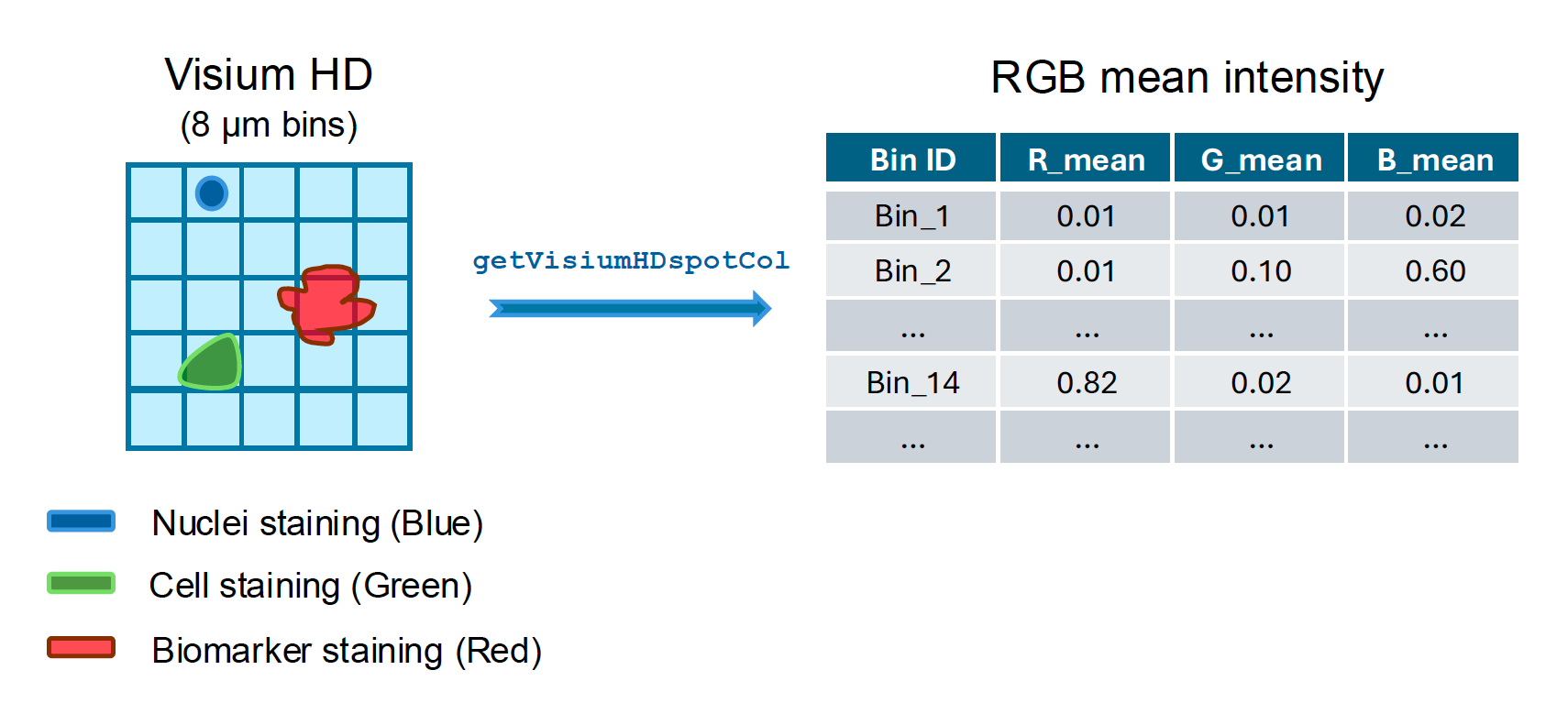
The getVisiumHDspotCol function: This function takes Visium HD data and an immunofluorescence (IF) image as input, calculates a matrix indicating the average Red, Green, and Blue color intensities in each bin. Users can select the bin size before the calculation.
9.3.1 Input prerequisites
To use the getVisiumHDspotCol function, users need to have the immunofluorescence staining image generated during the experiment. Such image may have multiple markers stained. For example, the following run includes the IF image associated with the Visium HD data through passing the jpg file using the colorizedimage parameter:
spaceranger count --id="WT-CO1" \
    --transcriptome=~/Data/Reference_files/refdata-gex-mm10-2020-A \
    --fastqs=~/Data/Fastq_files \
    --cytaimage=~/Data/Sample1.tif \
    --colorizedimage=~/Data/images_fluorescence/WT-CO1.jpg \
    --probe-set=~/Data/Reference_files/Visium_Mouse_Transcriptome_Probe_Set_v2.0_mm10-2020-A.csv \
    --slide=H1-ABDCEFJ \    #Using a random slide ID for illustration
    --area=A1 \
    --localcores=4 \
    --localmem=256 \
    --create-bam=false
After Space Ranger run, the images can be found in the spatial directory under the outs folder:
~/SpaceSequest/
  ├──src/
    ├── ...
    └── getVisiumHDspotCol.R

~/Data/WT-CO1/
  # High-resolution images
  ├── WT-CO1_IF_image_original.jpg

  # Space Ranger output
  ├── ...
  ├── binned_outputs/
  ├── cloupe_008um.cloupe
  ├── outs/
    ├── spatial/
    ├── aligned_fiducials.jpg
    ├── aligned_tissue_image.jpg
    ├── cytassist_image.tiff
    ├── detected_tissue_image.jpg
    ├── tissue_hires_image.png
    └── tissue_lowres_image.png
9.3.2 Run the function
library(Seurat)
library(ggplot2)
library(jpeg)
library(BiocParallel)
library(Matrix)

source("~/SpaceSequest/src/getVisiumHDspotCol.R")

#Input files
localdir <- "~/Data/WT-CO1/outs"
hires_image <- "~/Data/WT-CO1/outs/binned_outputs/square_008um/spatial
strImg <- "~/Data/WT-CO1/WT-CO1_IF_image_original.jpg"
prefix <- "WT-CO1"

#Process Visium HD data using Seurat 5
hires = Read10X_Image(hires_image, image.name = "tissue_hires_image.png")
object <- Load10X_Spatial(data.dir = localdir, bin.size = c(8), image = hires)
object@images[["slice1.008um"]]@scale.factors[["lowres"]] = object@images[["slice1.008um"]]@scale.factors[["hires"]]

#Run the function
#In an internal test dataset, this step took ~3 hours to run
cInfo <- getVisiumHDspotCol(object,strImg,core=4)
saveRDS(cInfo,paste0(prefix, ".alignImage.cInfo.rds"))

#Check the result
head(cInfo)
The result table has multiple columns, corresponding Red, Green, and Blue colors. For example, the Red color has three columns: R_mean, R_median, and R_sd, indicating the mean, median, and standard deviation of the Red color for each bin. In this example, the bin size was selected as 8 μm, but users can change it based on their need.